Black-oil model from scratch with history matching

Blackoil   StartToFinish   Introduction   HistoryMatching   Wells  

This script shows how to set up a black-oil model from scratch, using Jutul to set up the mesh and MultiComponentFlash to generate PVT tables. The script also shows how to set up a parametrized history matching problem and solve it using the optimize_reservoir function.

The purpose of this example is to have a "all in one" script that sets up all stages of a simulation model and a subsequent history matching workflow. The case itself is synthetic and not meant to be realistic, but it has enough complexity to show how to use the different pieces work together.

Define the mesh

We define a synthetic mesh by perturbing a Cartesian mesh, and then cutting it with a plane to create a fault. We also define a few layers in the vertical direction by assigning a layer index to each cell based on its depth. This will allow us to set different properties in each layer later on.

using Jutul, HYPRE, JutulDarcy, GeoEnergyIO, GLMakie, MultiComponentFlash, LinearAlgebra
nx = 60
ny = 40
nz = 10

L = 2000.0
W = 1000.0
H = 180.0
g_cart = CartesianMesh((nx, ny, nz), (L, W, H))
g = UnstructuredMesh(g_cart, z_is_depth = true)

for (idx, pt) in enumerate(g.node_points)
    x_norm, y_norm, z_norm = pt ./ (L, W, H)

    big_delta = cos(x_norm * π + 0.1)*1 + cos(y_norm * π/2  - 2*x_norm^2) * 1.2
    small_delta = x_norm*cos(y_norm * 8π) * 2 + cos(x_norm*y_norm * 5π) * 1
    tiny_noise = cos(y_norm * x_norm * 30π) * 0.5 + cos(y_norm * x_norm * 40π) * 0.5 + sin(x_norm * 30π) * sin(y_norm * x_norm * 30π)
    z_offset = 40*big_delta + 10*small_delta + 5*tiny_noise
    g.node_points[idx] = pt .+ (0.0, 0.0, z_offset)
end

geo = tpfv_geometry(g)

keep = Int[]
for c in Jutul.cells(g)
    x, y, z = geo.cell_centroids[:, c]
    x_norm, y_norm, z_norm = (x, y, z) ./ (L, W, H)
    if 0.5*(x_norm - 0.5 + 0.05*y_norm)^2 + 0.7x_norm*(y_norm - 0.5)^2 < 0.25^2
        push!(keep, c)
    end
end
g0 = g

UnstructuredMesh with 24000 cells, 68600 faces and 6800 boundary faces

Extract the active domain and add a fault

We extract a submesh to get a more interesting geometry, and then add a fault by cutting the mesh with a plane.

g = extract_submesh(g0, keep)

K = map(
    i -> cell_ijk(g, i)[3],
    Jutul.cells(g)
)

import Jutul.CutCellMeshes: PlaneCut, cut_mesh, cut_and_displace_mesh
cut = Jutul.CutCellMeshes.PlaneCut([2L/4, 250.0, 50.0], normalize([1.0, 0.4, -0.4]))
cutmesh, maps = cut_and_displace_mesh(g, cut;
        constant = 50.0,
        shift_lr = 10.0,
        side = :negative,
        face_tol = 1000.0,
        coplanar_tol = 1e-3,
        area_tol = 0.0,
        angle = 0.02,
        extra_out = true,
        min_cut_fraction = 0.0
)
g = cutmesh
K = K[maps[:cell_index]]

function k_to_layer(k)
    if k < 0.3*nz
        return 1
    elseif k < 0.7*nz
        return 2
    else
        return 3
    end
end

layer = k_to_layer.(K)
layer_to_cells = map(l -> findall(==(l), layer), 1:maximum(layer))

fig, ax, plt = plot_cell_data(g, layer)
plot_mesh_edges!(ax, g0)
fig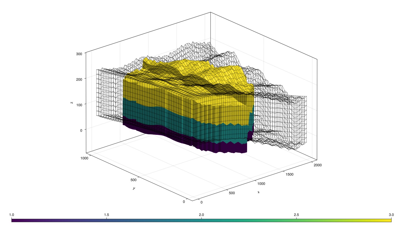

Set up a well configuration

As this script has variable nx/ny/nz, we can set up the wells using trajectories defined in physical space, instead of using cell indices. We set up 5 injectors and 3 producers. The injectors are in the boundary of the domain and are vertical, while the producers are horizontal and in the interior.

reservoir = reservoir_domain(g)
wells = []

t1 = [
    0.25 0.25 0;
    0.25 0.25 1.0
    ] .* [L, W, H]'

t2 = [
    0.22 0.5 0;
    0.22 0.5 1.0
    ] .* [L, W, H]'

t3 = [
    0.26 0.8 0;
    0.26 0.8 1.0
    ] .* [L, W, H]'

t4 = [
    0.66 0.25 0;
    0.66 0.25 1.0
    ] .* [L, W, H]'

t5 = [
    0.66 0.76 0;
    0.66 0.76 1.0
    ] .* [L, W, H]'


injector_trajectories = [t1, t2, t3, t4, t5]
injector_names = Symbol[]
for (i, traj) in enumerate(injector_trajectories)
    name = Symbol("I$i")
    push!(wells, setup_well_from_trajectory(reservoir, traj, name = name))
    push!(injector_names, name)
end

p1 = [
    0.38 0.6 0.36;
    0.4 0.8 0.37
    ] .* [L, W, H]'

p2 = [
    0.38 0.4 0.36;
    0.4 0.2 0.37
    ] .* [L, W, H]'

p3 = [
    0.45 0.55 0.36;
    0.6 0.55 0.37
    ] .* [L, W, H]'

producer_trajectories = [p1, p2, p3]
producer_names = Symbol[]
for (i, traj) in enumerate(producer_trajectories)
    name = Symbol("P$i")
    push!(wells, setup_well_from_trajectory(reservoir, traj, name = name))
    push!(producer_names, name)
end

fig, ax, plt = plot_mesh_edges(reservoir)
ax.zreversed[] = true
for w in wells
    plot_well!(ax, reservoir, w)
end

Generate PVT tables

We define a synthetic oil composition and use the MultiComponentFlash package to generate PVT tables for the oil and gas phases. We then use the setup_reservoir_model_from_blackoil_tables function to generate a black-oil model with the PVT tables, and specify that we want to include dissolved gas in the oil phase by setting disgas = true. If we set disgas = false, we would get an immiscible model instead, where the gas and oil phases do not interact. The default setup also includes a water/aqueous phase with defaulted properties.

data = [
    ("C1" ,     0.25)
    ("CO2",     0.005)
    ("N2" ,     0.005)
    ("C2" ,     0.03)
    ("C3" ,     0.01)
    ("C4" ,     0.2)
    ("C5" ,     0.2)
    ("C6" ,     0.3)
    ("C10",     0.5)
]

cnames = map(first, data)
z_oil = map(last, data)
z_oil = normalize(z_oil, 1)
mixture = MultiComponentMixture(cnames)
eos = GenericCubicEOS(mixture, PengRobinson())
T_res = convert_to_si(70.0, "Celsius")


tables = generate_pvt_tables(eos, z_oil, T_res;
    n_pvto = 10, n_pvdg = 10, n_undersaturated = 10)

PVTTableSet
============================================================
Saturation pressure: 4.4609e+06 Pa (44.61 bar) [bubble point (oil)]
------------------------------------------------------------
  pvto: PVTOTable (11 Rs levels)
  pvtg: nothing
  pvdg: PVDGTable (10 pressure points)
  pvdo: PVDOTable (20 pressure points)
Surface Densities
  Oil: 667.00 kg/m³
  Gas: 1.3823 kg/m³

Plot 1/B for the oil and gas phases

fig = Figure()
ax = Axis(fig[1, 1], title = "1/Bo", xlabel = "Pressure (bar)", ylabel = "1/Bo")
pvto = tables.pvto
for (p_i, Bo) in zip(pvto.p, pvto.Bo)
    lines!(ax, p_i./si_unit(:bar), 1 ./ Bo)
end
bo = 1 ./ map(first, tables.pvto.Bo)
p = tables.pvto.p_bub
lines!(ax, p./si_unit(:bar), bo)
xlims!(ax, 0.0, 120)

ax = Axis(fig[1, 2], title = "1/Bg", xlabel = "Pressure (bar)", ylabel = "1/Bg")
lines!(ax, tables.pvdg.p./si_unit(:bar), 1 ./ tables.pvdg.Bg)
xlims!(ax, 0.0, 120)
fig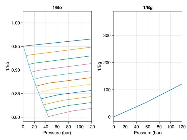

Generate the blackoil model with wells and PVT

We specify that we want to include dissolved gas (disgas = true) to allow gas to dissolve into the oil phase. Setting this to false would result in an immiscible model instead.

model = JutulDarcy.setup_reservoir_model_from_blackoil_tables(reservoir, tables, wells = wells, disgas = true)

MultiModel with 10 models and 32 cross-terms. 38800 equations, 38800 degrees of freedom and 101576 parameters.

  models:
    1) Reservoir (38736x38736)
       StandardBlackOilSystem with (AqueousPhase(), LiquidPhase(), VaporPhase())
       ∈ MinimalTPFATopology (12912 cells, 37796 faces)
    2) I1 (3x3)
       StandardBlackOilSystem with (AqueousPhase(), LiquidPhase(), VaporPhase())
       ∈ SimpleWell [I1] (1 nodes, 0 segments, 8 perforations)
    3) I2 (3x3)
       StandardBlackOilSystem with (AqueousPhase(), LiquidPhase(), VaporPhase())
       ∈ SimpleWell [I2] (1 nodes, 0 segments, 9 perforations)
    4) I3 (3x3)
       StandardBlackOilSystem with (AqueousPhase(), LiquidPhase(), VaporPhase())
       ∈ SimpleWell [I3] (1 nodes, 0 segments, 10 perforations)
    5) I4 (3x3)
       StandardBlackOilSystem with (AqueousPhase(), LiquidPhase(), VaporPhase())
       ∈ SimpleWell [I4] (1 nodes, 0 segments, 9 perforations)
    6) I5 (3x3)
       StandardBlackOilSystem with (AqueousPhase(), LiquidPhase(), VaporPhase())
       ∈ SimpleWell [I5] (1 nodes, 0 segments, 9 perforations)
    7) P1 (3x3)
       StandardBlackOilSystem with (AqueousPhase(), LiquidPhase(), VaporPhase())
       ∈ SimpleWell [P1] (1 nodes, 0 segments, 10 perforations)
    8) P2 (3x3)
       StandardBlackOilSystem with (AqueousPhase(), LiquidPhase(), VaporPhase())
       ∈ SimpleWell [P2] (1 nodes, 0 segments, 11 perforations)
    9) P3 (3x3)
       StandardBlackOilSystem with (AqueousPhase(), LiquidPhase(), VaporPhase())
       ∈ SimpleWell [P3] (1 nodes, 0 segments, 10 perforations)
    10) Facility (40x40)
       JutulDarcy.FacilitySystem{StandardBlackOilSystem{Tuple{Jutul.LinearInterpolant{Vector{Float64}, Vector{Float64}, @NamedTuple{x0::Float64, dx::Float64, n::Int64}}}, Nothing, true, Tuple{Float64, Float64, Float64}, :varswitch, @NamedTuple{a::Int64, l::Int64, v::Int64}, Tuple{AqueousPhase, LiquidPhase, VaporPhase}, Float64}}(StandardBlackOilSystem with (AqueousPhase(), LiquidPhase(), VaporPhase()))
       ∈ WellGroup([:I1, :I2, :I3, :I4, :I5, :P1, :P2, :P3], true, true)

  cross_terms:
    1) I1 <-> Reservoir (Eqs: mass_conservation <-> mass_conservation)
       JutulDarcy.ReservoirFromWellFlowCT
    2) I2 <-> Reservoir (Eqs: mass_conservation <-> mass_conservation)
       JutulDarcy.ReservoirFromWellFlowCT
    3) I3 <-> Reservoir (Eqs: mass_conservation <-> mass_conservation)
       JutulDarcy.ReservoirFromWellFlowCT
    4) I4 <-> Reservoir (Eqs: mass_conservation <-> mass_conservation)
       JutulDarcy.ReservoirFromWellFlowCT
    5) I5 <-> Reservoir (Eqs: mass_conservation <-> mass_conservation)
       JutulDarcy.ReservoirFromWellFlowCT
    6) P1 <-> Reservoir (Eqs: mass_conservation <-> mass_conservation)
       JutulDarcy.ReservoirFromWellFlowCT
    7) P2 <-> Reservoir (Eqs: mass_conservation <-> mass_conservation)
       JutulDarcy.ReservoirFromWellFlowCT
    8) P3 <-> Reservoir (Eqs: mass_conservation <-> mass_conservation)
       JutulDarcy.ReservoirFromWellFlowCT
    9) Facility  -> I1 (Eq: mass_conservation)
       JutulDarcy.WellFromFacilityFlowCT
    10) I1  -> Facility (Eq: bottom_hole_pressure_equation)
       JutulDarcy.FacilityFromWellBottomHolePressureCT
    11) I1  -> Facility (Eq: surface_phase_rates_equation)
       JutulDarcy.FacilityFromSurfacePhaseRatesCT
    12) Facility  -> I2 (Eq: mass_conservation)
       JutulDarcy.WellFromFacilityFlowCT
    13) I2  -> Facility (Eq: bottom_hole_pressure_equation)
       JutulDarcy.FacilityFromWellBottomHolePressureCT
    14) I2  -> Facility (Eq: surface_phase_rates_equation)
       JutulDarcy.FacilityFromSurfacePhaseRatesCT
    15) Facility  -> I3 (Eq: mass_conservation)
       JutulDarcy.WellFromFacilityFlowCT
    16) I3  -> Facility (Eq: bottom_hole_pressure_equation)
       JutulDarcy.FacilityFromWellBottomHolePressureCT
    17) I3  -> Facility (Eq: surface_phase_rates_equation)
       JutulDarcy.FacilityFromSurfacePhaseRatesCT
    18) Facility  -> I4 (Eq: mass_conservation)
       JutulDarcy.WellFromFacilityFlowCT
    19) I4  -> Facility (Eq: bottom_hole_pressure_equation)
       JutulDarcy.FacilityFromWellBottomHolePressureCT
    20) I4  -> Facility (Eq: surface_phase_rates_equation)
       JutulDarcy.FacilityFromSurfacePhaseRatesCT
    21) Facility  -> I5 (Eq: mass_conservation)
       JutulDarcy.WellFromFacilityFlowCT
    22) I5  -> Facility (Eq: bottom_hole_pressure_equation)
       JutulDarcy.FacilityFromWellBottomHolePressureCT
    23) I5  -> Facility (Eq: surface_phase_rates_equation)
       JutulDarcy.FacilityFromSurfacePhaseRatesCT
    24) Facility  -> P1 (Eq: mass_conservation)
       JutulDarcy.WellFromFacilityFlowCT
    25) P1  -> Facility (Eq: bottom_hole_pressure_equation)
       JutulDarcy.FacilityFromWellBottomHolePressureCT
    26) P1  -> Facility (Eq: surface_phase_rates_equation)
       JutulDarcy.FacilityFromSurfacePhaseRatesCT
    27) Facility  -> P2 (Eq: mass_conservation)
       JutulDarcy.WellFromFacilityFlowCT
    28) P2  -> Facility (Eq: bottom_hole_pressure_equation)
       JutulDarcy.FacilityFromWellBottomHolePressureCT
    29) P2  -> Facility (Eq: surface_phase_rates_equation)
       JutulDarcy.FacilityFromSurfacePhaseRatesCT
    30) Facility  -> P3 (Eq: mass_conservation)
       JutulDarcy.WellFromFacilityFlowCT
    31) P3  -> Facility (Eq: bottom_hole_pressure_equation)
       JutulDarcy.FacilityFromWellBottomHolePressureCT
    32) P3  -> Facility (Eq: surface_phase_rates_equation)
       JutulDarcy.FacilityFromSurfacePhaseRatesCT

Model storage will be optimized for runtime performance.

Define relative permeability curves

We define SWOF/SGOF tables to set the relative permeability curves. Here we use the Brooks-Corey model to generate the relperm points, but we could also have specified them manually or used a different model. Note that we set the connate water to zero by adding an additional point to the SWOF table before the first mobile point.

import JutulDarcy: brooks_corey_relperm
srw = 0.1
srow = 0.1
sw = collect(range(srw, 1.0 - srow, length = 20))
krw = brooks_corey_relperm.(sw, n = 2.0, residual = srw, residual_total = srow + srw)
kro = brooks_corey_relperm.(1 .- sw, n = 2.1, residual = srow, residual_total = srow + srw)

pushfirst!(sw, 0.0)
pushfirst!(krw, 0.0)
pushfirst!(kro, 1.0)
swof = hcat(sw, krw, kro)

srg = 0.0
srowg = 0.0
sg = range(srg, 1.0 - srowg, length = 20)
krg = brooks_corey_relperm.(sg, n = 2.1, residual = srg, residual_total = srowg + srg)
krog = brooks_corey_relperm.(1 .- sg, n = 1.8, residual = srowg, residual_total = srowg + srg)
sgof = hcat(sg, krg, krog)

set_relative_permeability!(model, swof = swof, sgof = sgof)

fig = Figure(size = (1200, 500))
ax = Axis(fig[1, 1], title = "Oil-water relperm", xlabel = "Sw", ylabel = "kr")
lines!(ax, swof[:, 1], swof[:, 2], label = "krw")
lines!(ax, swof[:, 1], swof[:, 3], label = "kro")
xlims!(ax, 0.0, 1.0)
axislegend(ax)
ax = Axis(fig[1, 2], title = "Gas relperm", xlabel = "Sg", ylabel = "kr")
lines!(ax, sgof[:, 1], sgof[:, 2], label = "krg")
lines!(ax, sgof[:, 1], sgof[:, 3], label = "krog")
xlims!(ax, 0.0, 1.0)
axislegend(ax)
fig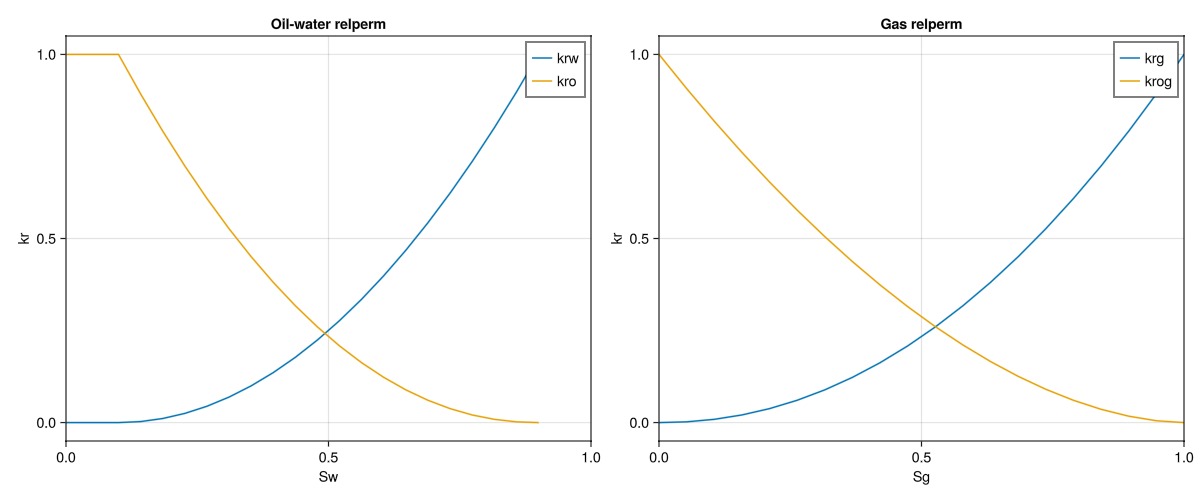

Equilibriate the model by setting fluid contacts

We define a single equilbrium region with datum pressure 110 bar at the depth of 0 meter (for simplicity, our model has zero depth at the top of the model instead of the surface). We set constant Rs, but could also have specified rs_vs_depth as a function to have a depth-dependent Rs. We also set the gas-oil contact (GOC) and water-oil contact (WOC) to be at 30% and 80% of the total initial height of the model, respectively.

eql = EquilibriumRegion(model, si"110bar", si"0meter",
    goc = 0.3*H,
    woc = 0.8*H,
    rs = 40.0
)
state0 = setup_reservoir_state(model, eql);

Set up schedule

total_time = si"20year"

one_pvi = sum(pore_volume(reservoir)) / total_time
injector_rate = 0.8*one_pvi/length(injector_names)
producer_rate = 0.8*one_pvi/length(producer_names)

n_steps = 40
dt = fill(total_time/n_steps, n_steps)

40-element Vector{Float64}:
 1.5778476e7
 1.5778476e7
 1.5778476e7
 1.5778476e7
 1.5778476e7
 1.5778476e7
 1.5778476e7
 1.5778476e7
 1.5778476e7
 1.5778476e7
 ⋮
 1.5778476e7
 1.5778476e7
 1.5778476e7
 1.5778476e7
 1.5778476e7
 1.5778476e7
 1.5778476e7
 1.5778476e7
 1.5778476e7

dt = dt[1:1]

forces = []
for (i, dt_i) in enumerate(dt)
    t = sum(dt[1:i])
    control = Dict()
    for name in injector_names
        control[name] = setup_injector_control(injector_rate, :wrat, [1.0, 0.0, 0.0], density = 1000.0)
    end
    for name in producer_names
        control[name] = setup_producer_control(si"90bar", :bhp)
    end
    f = setup_reservoir_forces(model, control = control)
    push!(forces, f)
end

Parametrize the model and define a truth case

We set a few parameters that we want to tune in the history matching process, and define a "truth case" by setting these parameters to specific values and simulating the model. The parameters we choose to define the model are the porosity and permeability of each layer, the multiplier on the transmissibilities of the fault faces, and the vertical/horizontal permeability ratio (kv_ratio). We could also have used setup_reservoir_dict_optimization to make a setup function automatically that exposes "standard" parameters.

truth_prm = Dict(
    "LAYER_PORO" => [0.15, 0.22, 0.10],
    "LAYER_PERM" => [200.0, 800.0, 100.0],
    "FAULT_MULTIPLIER" => 0.1,
    "KV_RATIO" => 0.1
)

nc = number_of_cells(reservoir)
nlayers = maximum(layer)
fault_faces = maps[:new_faces]

function setup_my_blackoil_model(prm, step_info = missing)
    layer_poro = prm["LAYER_PORO"]
    layer_perm = prm["LAYER_PERM"]
    fault_multiplier = prm["FAULT_MULTIPLIER"]
    kv_ratio = prm["KV_RATIO"]
    num_type = promote_type(eltype(layer_poro), eltype(layer_perm), typeof(fault_multiplier), typeof(kv_ratio))

    updated_model = deepcopy(model)
    updated_reservoir = reservoir_domain(updated_model)

    new_perm = zeros(num_type, 3, nc)
    new_poro = zeros(num_type, nc)
    for l in 1:nlayers
        cells = layer_to_cells[l]
        layer_k = layer_perm[l] * si_unit("millidarcy")
        new_perm[1, cells] .= layer_k
        new_perm[2, cells] .= layer_k
        new_perm[3, cells] .= layer_k * kv_ratio
        new_poro[cells] .= layer_poro[l]
    end
    updated_reservoir[:permeability] = new_perm
    updated_reservoir[:porosity] = new_poro

    new_parameters = deepcopy(setup_parameters(updated_model))
    trans = new_parameters[:Reservoir][:Transmissibilities]
    trans = num_type.(trans)
    trans[fault_faces] .*= fault_multiplier
    new_parameters[:Reservoir][:Transmissibilities] = trans
    return JutulCase(updated_model, dt, forces; parameters = new_parameters, state0 = deepcopy(state0))
end

truth_case = setup_my_blackoil_model(truth_prm)
truth_sim = simulate_reservoir(truth_case)

ReservoirSimResult with 40 entries:

  wells (8 present):
    :I5
    :I3
    :P1
    :I4
    :I2
    :P3
    :I1
    :P2
    Results per well:
       :wrat => Vector{Float64} of size (40,)
       :Aqueous_mass_rate => Vector{Float64} of size (40,)
       :orat => Vector{Float64} of size (40,)
       :bhp => Vector{Float64} of size (40,)
       :mrat => Vector{Float64} of size (40,)
       :gor => Vector{Float64} of size (40,)
       :lrat => Vector{Float64} of size (40,)
       :mass_rate => Vector{Float64} of size (40,)
       :rate => Vector{Float64} of size (40,)
       :Vapor_mass_rate => Vector{Float64} of size (40,)
       :control => Vector{Symbol} of size (40,)
       :Liquid_mass_rate => Vector{Float64} of size (40,)
       :wcut => Vector{Float64} of size (40,)
       :grat => Vector{Float64} of size (40,)

  states (Vector with 40 entries, reservoir variables for each state)
    :Pressure => Vector{Float64} of size (12912,)
    :ImmiscibleSaturation => Vector{Float64} of size (12912,)
    :BlackOilUnknown => Vector{BlackOilX{Float64}} of size (12912,)
    :TotalMasses => Matrix{Float64} of size (3, 12912)
    :Rs => Vector{Float64} of size (12912,)
    :Saturations => Matrix{Float64} of size (3, 12912)

  time (report time for each state)
     Vector{Float64} of length 40

  result (extended states, reports)
     SimResult with 40 entries

  extra
     Dict{Any, Any} with keys :simulator, :config

  Completed at Mar. 18 2026 13:34 after 48 seconds, 87 milliseconds, 722.9 microseconds.

Plot the results of the truth case

truth_summary = truth_sim.summary
JutulDarcy.plot_summary(truth_summary, plots = ["FOPR,FWPR,FGPR", "FOPT,FWPT,FGPT", "FPR", "FOIP"], unit_system = "Field", cols = 2)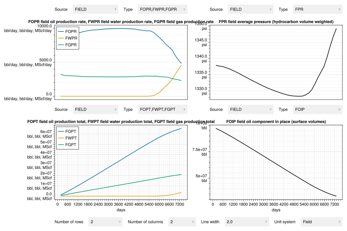

Plot the well results

plot_well_results(truth_sim.wells)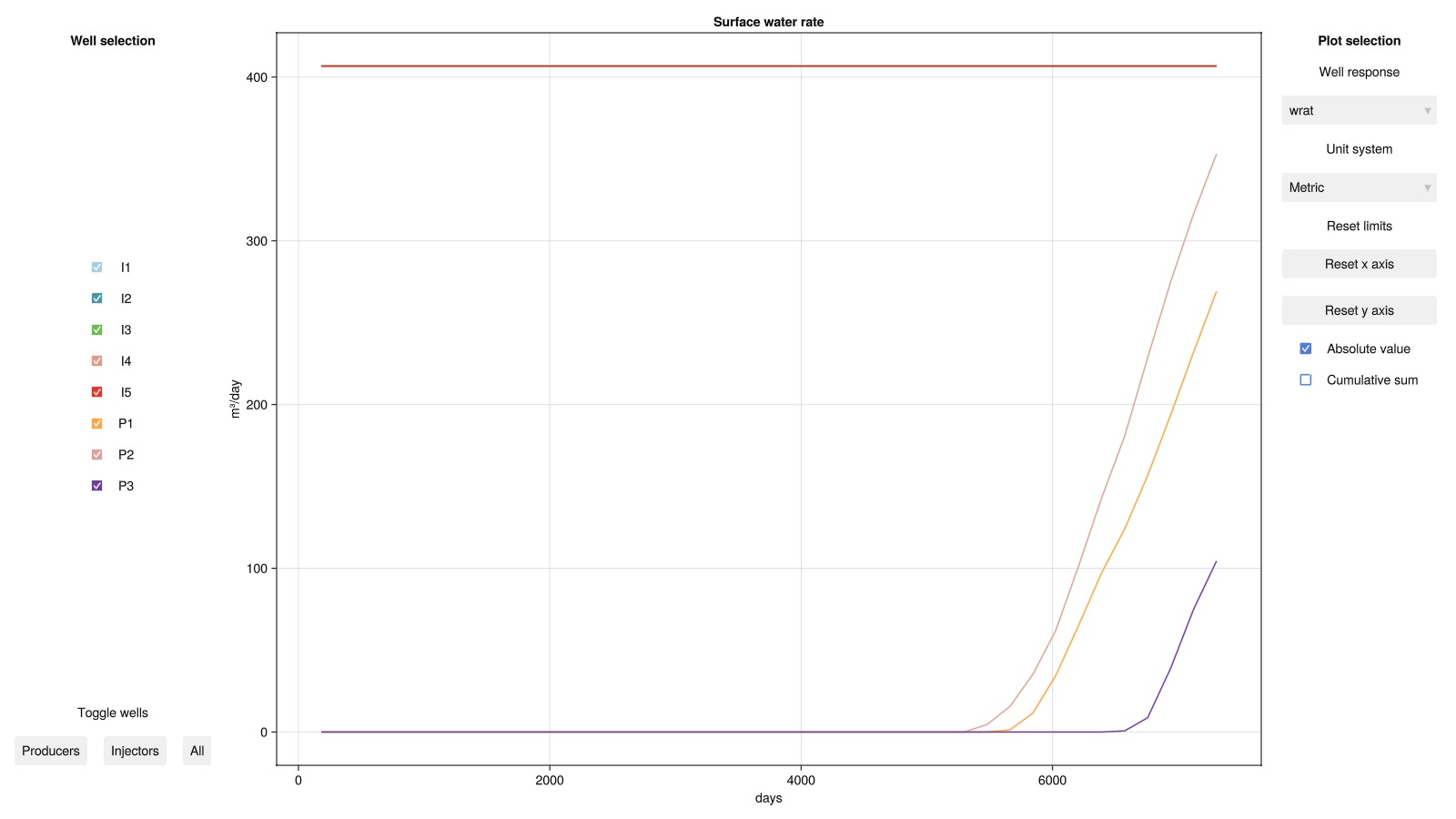

Plot the reservoir results

reservoir = reservoir_domain(truth_case)
ex = plot_explorer(reservoir, dynamic = truth_sim.states,
    colormap = :seaborn_icefire_gradient,
    zreversed = true
)
for w in wells
    plot_well!(ex.lscene, reservoir, w)
end
ex.fig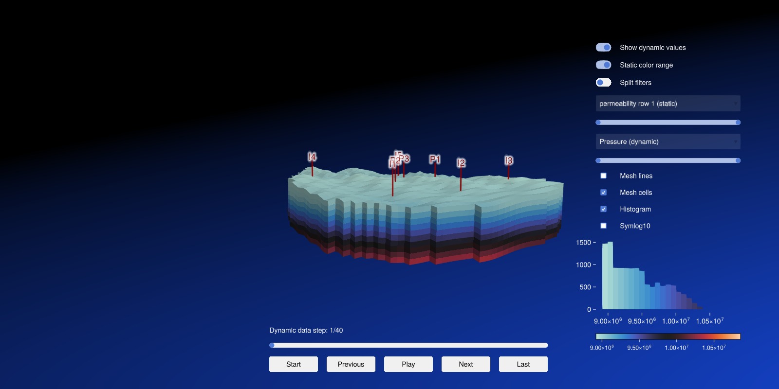

Define an initial guess that is different from the truth case

initial_prm = Dict(
    "LAYER_PORO" => [0.1, 0.1, 0.1],
    "LAYER_PERM" => [100.0, 100.0, 100.0],
    "FAULT_MULTIPLIER" => 1.0,
    "KV_RATIO" => 0.1
)

initial_case = setup_my_blackoil_model(initial_prm)
initial_sim = simulate_reservoir(initial_case)
JutulDarcy.plot_summary([truth_summary, initial_sim.summary], names = ["Truth", "Initial model"], plots = ["FOPR,FWPR,FGPR", "FOPT,FWPT,FGPT", "FPR", "FOIP"], unit_system = "Field", cols = 2)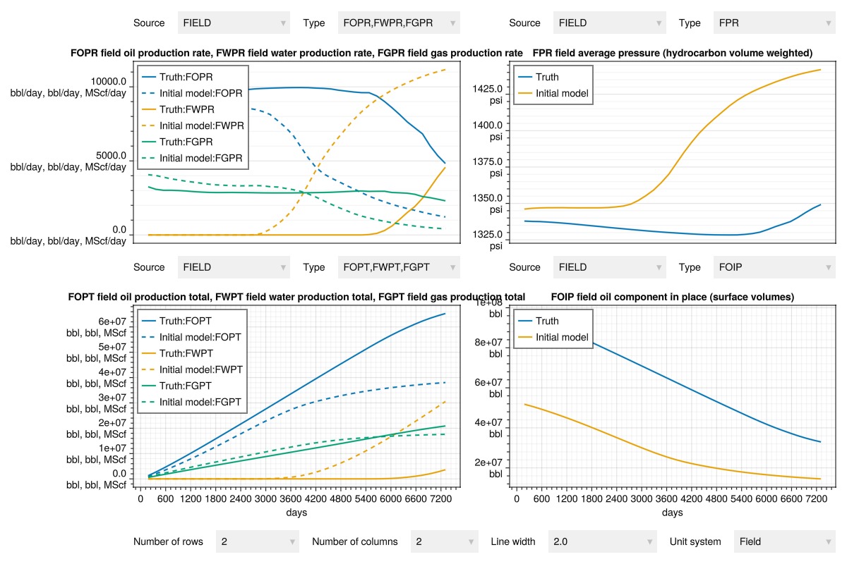

Define a history match objective and evaluate the mismatch of the initial guess

import JutulDarcy.HistoryMatching: match_injectors!, match_producers!, history_match_objective, evaluate_match

obj = history_match_objective(truth_case, truth_sim)
match_producers!(obj, :orat, weight = 1.0)
match_producers!(obj, :lrat, weight = 1.0)
match_injectors!(obj, :bhp, weight = 4.0)
display(obj)
JutulDarcy.plot_mismatch(obj, initial_sim)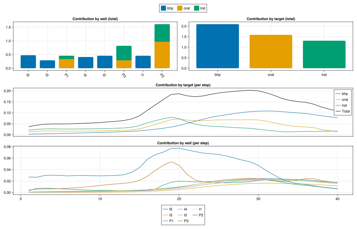

Set up the optimization problem and solve

dopt = Jutul.DictOptimization.DictParameters(initial_prm, setup_my_blackoil_model)
free_optimization_parameter!(dopt, "LAYER_PORO", abs_min = 0.10, abs_max = 0.25)
free_optimization_parameter!(dopt, "LAYER_PERM", abs_min = 100.0, abs_max = 1000.0, scaler = :log)
free_optimization_parameter!(dopt, "FAULT_MULTIPLIER", abs_min = 0.01, abs_max = 1.0, initial = 0.5)

display(dopt)

Run the history matching

We use the built-in optimizer to run a few iterations of matching. The adjoint method calculates gradients for us.

tuned_prm = optimize_reservoir(dopt, obj;
    allow_errors = true,
    max_it = 15,
    lbfgs_num = 25,
    ls_max_it = 3,
    optimizer = :lbfgsb_qp
)

Dict{String, Any} with 4 entries:
  "FAULT_MULTIPLIER" => 0.522522
  "LAYER_PERM"       => [100.0, 260.165, 130.745]
  "KV_RATIO"         => 0.1
  "LAYER_PORO"       => [0.1, 0.1842, 0.25]

Evaluate the tuned model and compare to truth and initial guess

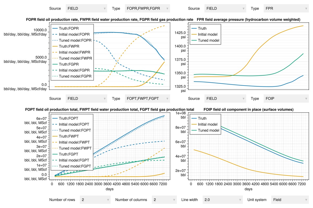
Note that the optimization reduces the mismatch significantly, but the tuned model is still different from the truth case. This is a result of the non-uniqueness of the problem, where different parameter combinations can give similar responses.

tuned_case = setup_my_blackoil_model(tuned_prm)
tuned_sim = simulate_reservoir(tuned_case)
# Plot the results of the tuned model compared to the truth and initial guess
JutulDarcy.plot_summary(
    [truth_summary, initial_sim.summary, tuned_sim.summary],
    names = ["Truth", "Initial model", "Tuned model"],
    plots = ["FOPR,FWPR,FGPR", "FOPT,FWPT,FGPT", "FPR", "FOIP"],
    unit_system = "Field",
    cols = 2
)

Example on GitHub

If you would like to run this example yourself, it can be downloaded from the JutulDarcy.jl GitHub repository as a script, or as a Jupyter Notebook

This example took 1988.653203036 seconds to complete.

---

This page was generated using Literate.jl.