Adjoint gradients for the SPE1 model

This is a brief example of how to set up a case and compute adjoint gradients for the SPE1 model in a few different ways. These techniques are in general applicable to DATA-type models.

Load the model

using Jutul, JutulDarcy, GeoEnergyIO, GLMakie
data_pth = joinpath(GeoEnergyIO.test_input_file_path("SPE1"), "SPE1.DATA")
data = parse_data_file(data_pth);
case = setup_case_from_data_file(data);

Set up a function to set up the case with custom porosity

We create a setup function that takes in a parameter dictionary prm and returns a case with the porosity set to the value in prm["poro"]. This is a convenient way to customize a case prior to setup, allowing direct interaction with keywords like PERMX, PORO, etc.

function F(prm, step_info = missing)
    data_c = deepcopy(data)
    data_c["GRID"]["PORO"] = fill(prm["poro"], size(data_c["GRID"]["PORO"]))
    case = setup_case_from_data_file(data_c)
    return case
end

F (generic function with 2 methods)

Define and simulate truth case (poro from input)

x_truth = only(unique(data["GRID"]["PORO"]))
prm_truth = Dict("poro" => x_truth)
case_truth = F(prm_truth)
ws, states = simulate_reservoir(case_truth)

ReservoirSimResult with 120 entries:

  wells (2 present):
    :INJ
    :PROD
    Results per well:
       :wrat => Vector{Float64} of size (120,)
       :Aqueous_mass_rate => Vector{Float64} of size (120,)
       :orat => Vector{Float64} of size (120,)
       :bhp => Vector{Float64} of size (120,)
       :gor => Vector{Float64} of size (120,)
       :lrat => Vector{Float64} of size (120,)
       :mass_rate => Vector{Float64} of size (120,)
       :rate => Vector{Float64} of size (120,)
       :Vapor_mass_rate => Vector{Float64} of size (120,)
       :control => Vector{Symbol} of size (120,)
       :Liquid_mass_rate => Vector{Float64} of size (120,)
       :wcut => Vector{Float64} of size (120,)
       :grat => Vector{Float64} of size (120,)

  states (Vector with 120 entries, reservoir variables for each state)
    :Pressure => Vector{Float64} of size (300,)
    :ImmiscibleSaturation => Vector{Float64} of size (300,)
    :BlackOilUnknown => Vector{BlackOilX{Float64}} of size (300,)
    :TotalMasses => Matrix{Float64} of size (3, 300)
    :Rs => Vector{Float64} of size (300,)
    :Saturations => Matrix{Float64} of size (3, 300)

  time (report time for each state)
     Vector{Float64} of length 120

  result (extended states, reports)
     SimResult with 120 entries

  extra
     Dict{Any, Any} with keys :simulator, :config

  Completed at Jul. 06 2025 18:07 after 1 second, 601 milliseconds, 894 microseconds.

Define pressure difference as objective function

function pdiff(p, p0)
    v = 0.0
    for i in eachindex(p)
        v += (p[i] - p0[i])^2
    end
    return v
end

step_times = cumsum(case.dt)
total_time = step_times[end]
function mismatch_objective(m, s, dt, step_info, forces)
    t = step_info[:time] + dt
    step = findmin(x -> abs(x - t), step_times)[2]
    p = s[:Reservoir][:Pressure]
    v = pdiff(p, states[step][:Pressure])
    return (dt/total_time)*(v/(si_unit(:bar)*100)^2)
end

mismatch_objective (generic function with 1 method)

Create a perturbed initial guess and optimize

We create a perturbed initial guess for the porosity and optimize the case using the mismatch objective function defined above. The optimization will adjust the porosity to minimize the mismatch between the simulated pressure and the truth case, and recover the original porosity value of 0.3.

prm = Dict("poro" => x_truth .+ 0.25)
dprm = setup_reservoir_dict_optimization(prm, F)
free_optimization_parameter!(dprm, "poro", abs_max = 1.0, abs_min = 0.1)
prm_opt = optimize_reservoir(dprm, mismatch_objective);
dprm

DictParameters with 1 active parameters and 0 inactive:
Active optimization parameters
┌──────┬───────────────┬───────┬─────┬─────┬─────────────────┬────────┐
│ Name │ Initial value │ Count │ Min │ Max │ Optimized value │ Change │
├──────┼───────────────┼───────┼─────┼─────┼─────────────────┼────────┤
│ poro │ 0.55          │     1 │ 0.1 │ 1.0 │ 0.3             │ -45.0% │
└──────┴───────────────┴───────┴─────┴─────┴─────────────────┴────────┘
No inactive optimization parameters.

Plot the optimization history

using GLMakie
fig = Figure()
ax = Axis(fig[1, 1], xlabel = "LBFGS iteration", ylabel = "Objective function", yscale = log10)
scatter!(ax, dprm.history.val)
fig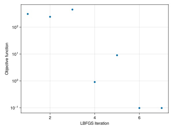

Use lumping to match permeability

The model contains three layers with different permeability. We can perturb the permeability in each layer a bit and use the lumping and scaling functionality in the optimizer to recover the original values.

We first define the setup function which expands a permeability value in each cell to PERMX, PERMY and PERMZ, as these are equal for the base model.

rmesh = physical_representation(reservoir_domain(case.model))
layerno = map(i -> cell_ijk(rmesh, i)[3], 1:number_of_cells(rmesh))
darcy = si_unit(:darcy)

function F_perm(prm, step_info = missing)
    data_c = deepcopy(data)
    sz = size(data_c["GRID"]["PERMX"])
    permxyz = reshape(prm["perm"], sz)
    data_c["GRID"]["PERMX"] = permxyz
    data_c["GRID"]["PERMY"] = permxyz
    data_c["GRID"]["PERMZ"] = permxyz
    case = setup_case_from_data_file(data_c)
    return case
end

F_perm (generic function with 2 methods)

Define the starting point

We perturb each layer a bit by multiplying with a constant factor to create a case where the pressure matches.

perm_truth = vec(data["GRID"]["PERMX"])
factors = [1.5, 2.0, 5.0]
prm = Dict(
    "perm" => perm_truth.*factors[layerno],
)

Dict{String, Vector{Float64}} with 1 entry:
  "perm" => [7.40192e-13, 7.40192e-13, 7.40192e-13, 7.40192e-13, 7.40192e-13, 7…

Optimize with lumping

We can lump parameters of the same name together. In this case, "perm" has one value per cell. We would like to exploit the fact that we know that there should be one unique value per layer as a prior assumption.

We already have a vector with one entry per cell that defines the layers, so we can use this as the lumping parameter directly.

perm_opt = setup_reservoir_dict_optimization(prm, F_perm)
free_optimization_parameter!(perm_opt, "perm", rel_min = 0.1, rel_max = 10.0, lumping = layerno)
perm_tuned = optimize_reservoir(perm_opt, mismatch_objective);
perm_opt

DictParameters with 1 active parameters and 0 inactive:
Active optimization parameters
┌──────┬─────────────────────────────┬───────┬─────────────────────────────┬────
│ Name │ Initial value               │ Count │                         Min │   ⋯
├──────┼─────────────────────────────┼───────┼─────────────────────────────┼────
│ perm │ 7.4e-13, 9.87e-14, 9.87e-13 │     3 │ 7.4e-14, 9.87e-15, 9.87e-14 │ 7 ⋯
└──────┴─────────────────────────────┴───────┴─────────────────────────────┴────
                                                               3 columns omitted
No inactive optimization parameters.

Plot the recovered permeability

first_entry = map(i -> findfirst(isequal(i), layerno), 1:3)
kval = [perm_truth[first_entry]..., prm["perm"][first_entry]..., perm_tuned["perm"][first_entry]...]
kval = 1000.0.*kval./si_unit(:darcy)
catval = [1, 2, 3, 1, 2, 3, 1, 2, 3]
group = [1, 1, 1, 2, 2, 2, 3, 3, 3]

colors = Makie.wong_colors()
fig, ax, plt = barplot(catval, kval,
    dodge = group,
    color = colors[group],
    axis = (
        xticks = (1:3, ["Layer 1", "Layer 2", "Layer 3"]),
        ylabel = "Permeability / md",
        title = "Tuned permeability layers"
    ),
)
labels = ["Truth", "Initial guess", "Optimized"]
elements = [PolyElement(polycolor = colors[i]) for i in 1:length(labels)]
title = "Categories"
Legend(fig[1,2], elements, labels, title)
fig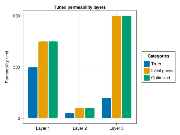

Compute sensitivities outside the optimization

We can also compute the sensitivities outside the optimization process. As our previous setup funciton only has a single parameter (the porosity), we instead switch to the setup_reservoir_dict_optimization function that can set up a set of "typical" tunable parameters for any reservoir model. This saves us the hassle of writing this function ourselves when we want to optimize e.g. permeability, porosity and well indices.

dprm_case = setup_reservoir_dict_optimization(case)
free_optimization_parameters!(dprm_case)
dprm_grad = parameters_gradient_reservoir(dprm_case, mismatch_objective);

setup_reservoir_state: Received primary variable LiquidSaturation, but this is not known to reservoir model.
setup_reservoir_state: Received primary variable VaporSaturation, but this is not known to reservoir model.
Optimization: Setting up adjoint storage.
Optimization: Finished setup in 10.472092551 seconds.

Plot the gradient of the mismatch objective with respect to the porosity

We see, as expected, that the gradient is largest in magnitude around the wells and near the front of the displacement.

m = physical_representation(reservoir_domain(case.model))
fig, ax, plt = plot_cell_data(m, dprm_grad[:model][:porosity])
ax.title[] = "Gradient of mismatch objective with respect to porosity"
fig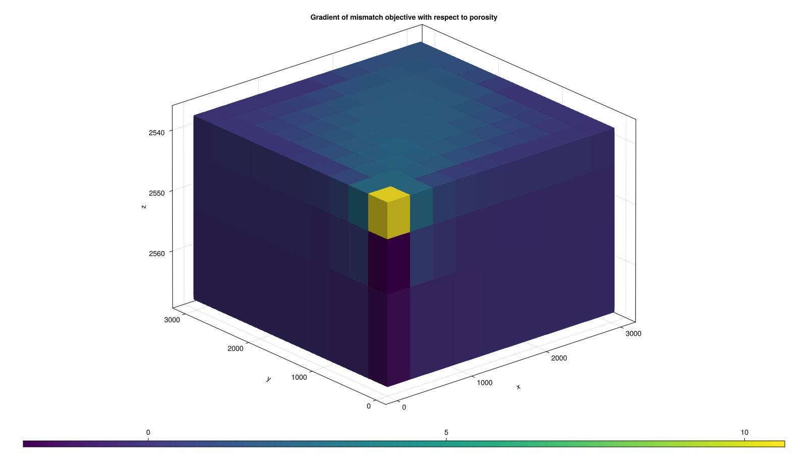

Plot the sensitivities in the interactive viewer

If you are running the example yourself, you can now explore the sensitivities in the interactive viewer. This is useful for understanding how the model responds to changes in the parameters.

plot_reservoir(case.model, dprm_grad[:model])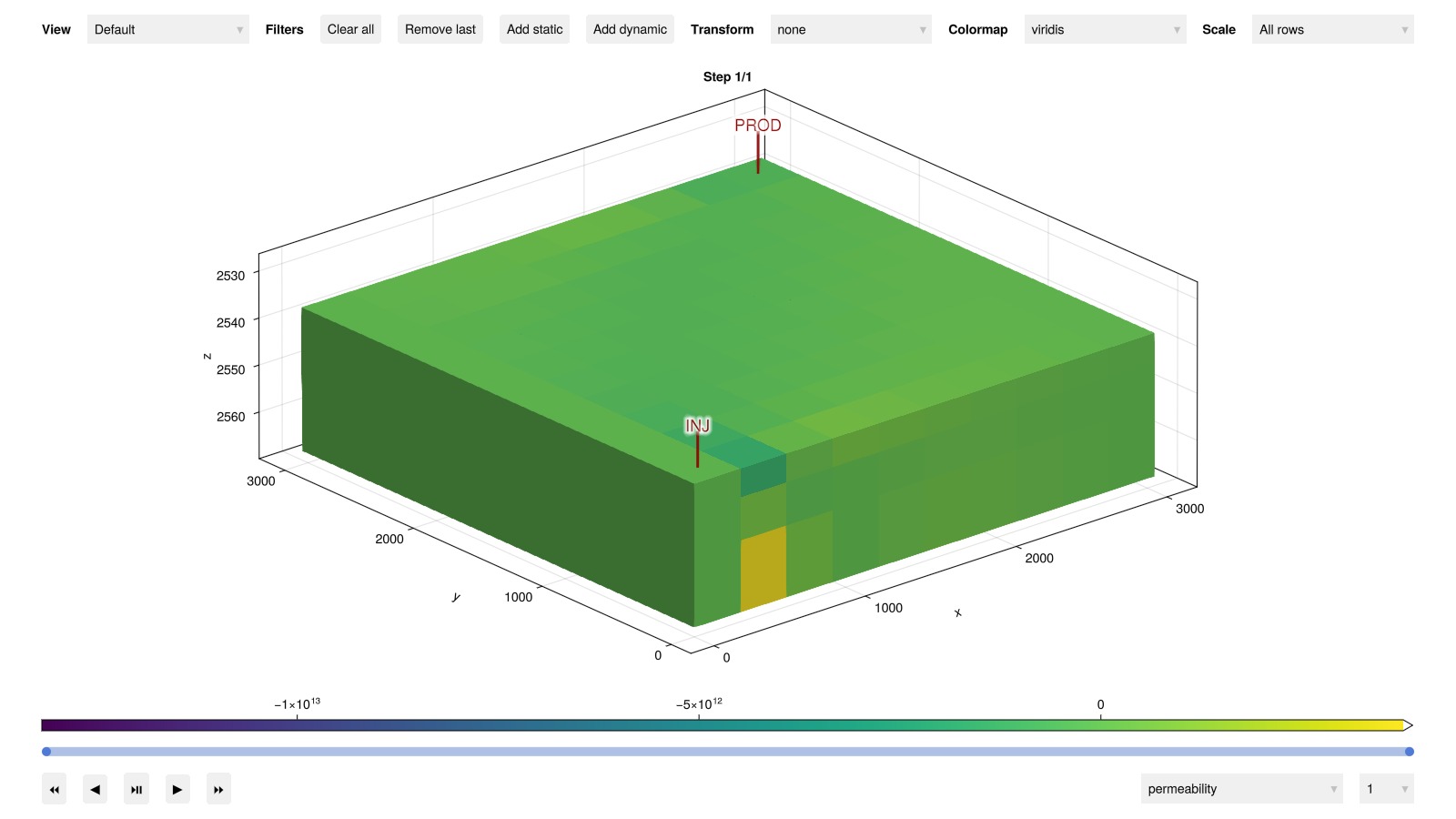

Example on GitHub

If you would like to run this example yourself, it can be downloaded from the JutulDarcy.jl GitHub repository as a script, or as a Jupyter Notebook

This example took 228.938251548 seconds to complete.

---

This page was generated using Literate.jl.