Borehole Thermal Energy Storage (BTES)
Geothermal Introduction MeshingThis script demonstrates how to model a borehole thermal energy storage (BTES) system using JutulDarcy. We will set up a BTES system with 50 wells, and simulate five year of operation with 6 months of charging followed by 6 months of discharging.
using Jutul, JutulDarcy
using LinearAlgebra
using HYPRE
using GLMakie
import Gmsh: gmsh
import Dates: monthname

atm, kilogram, meter, Kelvin, joule, watt, litre, year, second, darcy =
    si_units(:atm, :kilogram, :meter, :Kelvin, :joule, :watt, :litre, :year, :second, :darcy)
(101325.0, 1.0, 1.0, 1.0, 1.0, 1.0, 0.001, 3.1556952e7, 1.0, 9.86923266716013e-13)Define BTES well coordinates
We place the BTES wells in a pattern inspired by sunflower seeds, ensuring that they are uniformy distributed over the domain.
num_wells = 50
radius = 15.0meter
φ = (1 + sqrt(5))/2 # Golden ratio
Δθ = 2*π/φ^2
p = (k) -> radius .* sqrt(k/num_wells) .* (cos(k*Δθ), sin(k*Δθ))
well_coords = [p(k) for k = 0:num_wells-1];
Plot well coordinates in horizontal plane
fig = Figure()
ax = Axis(fig[1, 1], title = "BTES well coordinates", aspect = 1.0)
scatter!(ax, well_coords, markersize=10)
fig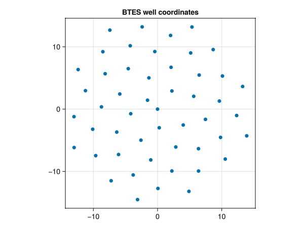
Set up mesh function
We create a mesh for the BTES system using Gmsh. The mesh is first created in 2D with refinement around the wells, and then extruded to create a 3D mesh.
function create_btes_mesh(xw, radius, depth, h_min, h_max, h_z)

    radius_outer = radius*5

    gmsh.initialize()
    gmsh.clear()
    gmsh.model.add("btes_mesh")

    perimeter = 2*π*radius_outer
    n = Int(ceil(perimeter / h_max))
    Δθ = 2*π/n
    for i = 1:n
        x, y = radius_outer*cos(i*Δθ), radius_outer*sin(i*Δθ)
        gmsh.model.geo.addPoint(x, y, 0.0, h_max, i)
    end
    for i = 1:n
        gmsh.model.geo.addLine(i, mod(i, n) + 1, i)
    end
    gmsh.model.geo.addCurveLoop(collect(1:n), 1)
    gmsh.model.geo.addPlaneSurface([1], 1)

    for (i, x) in enumerate(xw)
        gmsh.model.geo.addPoint(x[1], x[2], 0.0, h_min, n + i)
    end
    nw = length(xw)
    gmsh.model.geo.synchronize()
    gmsh.model.mesh.embed(0, collect(n+1:n+length(xw)), 2, 1)
    gmsh.model.geo.addPoint(0.0, 0.0, 0.0, h_min, n + nw + 1)

    gmsh.model.mesh.field.add("Distance", 1)
    gmsh.model.mesh.field.setNumbers(1, "PointsList", [n + nw + 1])
    gmsh.model.mesh.field.add("Threshold", 2)
    gmsh.model.mesh.field.setNumber(2, "InField", 1)
    gmsh.model.mesh.field.setNumber(2, "SizeMin", h_min)
    gmsh.model.mesh.field.setNumber(2, "SizeMax", h_max)
    gmsh.model.mesh.field.setNumber(2, "DistMin", 1.1*radius)
    gmsh.model.mesh.field.setNumber(2, "DistMax", 1.5*radius)
    gmsh.model.mesh.field.setAsBackgroundMesh(2)

    gmsh.model.geo.mesh.setRecombine(2, 1)

    num_elements = Int(ceil(depth/h_z))
    gmsh.model.geo.extrude([(2, 1)], 0, 0, depth, [num_elements], [1.0], true)
    gmsh.model.geo.synchronize()

    gmsh.model.mesh.generate(3)

    mesh = Jutul.mesh_from_gmsh(z_is_depth=true)
    gmsh.finalize()
    return mesh

end
create_btes_mesh (generic function with 1 method)Create BTES mesh
The following mesh size parameters will give a mesh with approximately 15k cells, and can be adjusted to make the mesh coarser or finer. NB: Note that not all mesh sizes will give a valid mesh.
depth = 50.0meter; # Depth of the BTES systemHorizontal minimum/maximum and vertical mesh size
h_min, h_max, h_z = 1.0meter, 25.0meter, 5.0meter
mesh = create_btes_mesh(well_coords, radius, depth, h_min, h_max, h_z)
UnstructuredMesh with 13170 cells, 38003 faces and 3014 boundary facesCreate reservoir model
We construct a simulation model with shallow bedrock posed on the mesh we just created and add the BTES wells.
Reservoir domain
The eservoir domain is populated with rock properties similar to that of granite
domain = reservoir_domain(mesh,
    permeability = 1e-6darcy,
    porosity = 0.011,
    rock_density = 2650kilogram/meter^3,
    rock_heat_capacity = 790joule/kilogram/Kelvin,
    rock_thermal_conductivity = 3.0watt/meter/Kelvin,
    component_heat_capacity = 4.278e3joule/kilogram/Kelvin
);
Set up BTES wells
The BTES well have a U-tube configuration, where the supply and return pipes run parallel inside a larger borehole filled with grout. We model this using two mutlisegment wells, one for the supply and one for the return. Pipe dimensions and material thermal properties have reasonable defaults, and can be adjusted as needed – see setup_btes_well for detail.
grid = physical_representation(domain)
well_models = []
for (wno, xw) in enumerate(well_coords)
    d = max(norm(xw, 2))
    v = (d > 0) ? xw ./ d : (1.0, 0.0)
    xw = xw .+ (h_min / 2) .* v
    trajectory = [xw[1] xw[2] 0.0; xw[1] xw[2] depth]
    cells = Jutul.find_enclosing_cells(grid, trajectory)
    name = Symbol("B$wno")
    w_sup, w_ret = setup_btes_well(domain, cells, name=name, btes_type=:u1)
    push!(well_models, w_sup, w_ret)
end
Make the model
model = setup_reservoir_model(
    domain, :geothermal,
    wells=well_models
);
Inspect
plot_reservoir(model)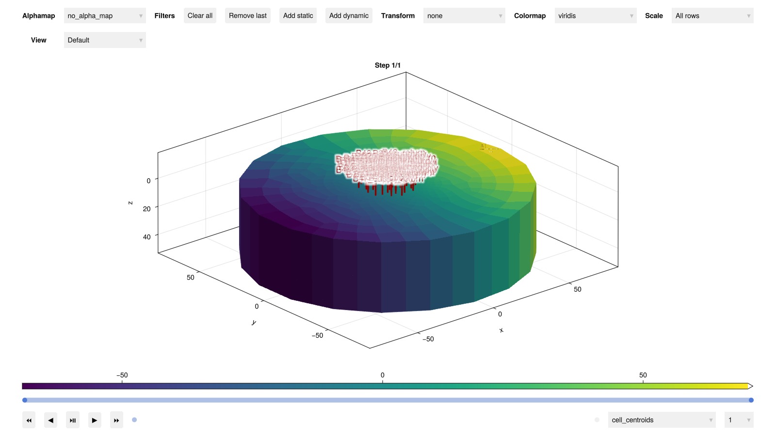
Initial state and boundary conditions
The model is initialized at 1 atm and 10°C.
state0 = setup_reservoir_state(model,
    Pressure=1atm,
    Temperature=convert_to_si(10.0, :Celsius)
);
We impose fixed boundary conditions at the top surface, enforcing a constant pressure of 1 atm and a temperature of 10°C.
geo = tpfv_geometry(mesh)
z_f = geo.boundary_centroids[3, :]
top_f = findall(v -> isapprox(v, minimum(z_f)), z_f)
top = mesh.boundary_faces.neighbors[top_f]
bc = FlowBoundaryCondition.(top, 1atm, convert_to_si(10.0, :Celsius));
Controls
The supply well of each BTES is controlled by a rate target, while the return well is controlled by a BHP target. The supply and return wells communicate through their bottom cell.
Rate control for supply side:
rate = 0.5litre/second
temperature_charge = convert_to_si(80.0, :Celsius)
temperature_discharge = convert_to_si(10.0, :Celsius)
rate_target = TotalRateTarget(rate)
ctrl_charge = InjectorControl(rate_target, [1.0], density=1000.0, temperature=temperature_charge)
ctrl_discharge = InjectorControl(rate_target, [1.0], density=1000.0, temperature=temperature_discharge);
BHP control for return side:
bhp_target = BottomHolePressureTarget(1atm)
ctrl_prod = ProducerControl(bhp_target);
Set up forces
control_charge = Dict()
control_discharge = Dict()
for welld in well_models
    well = physical_representation(welld)
    if contains(String(well.name), "_supply")
        control_charge[well.name] = ctrl_charge
        control_discharge[well.name] = ctrl_discharge
    else
        control_charge[well.name] = ctrl_prod
        control_discharge[well.name] = ctrl_prod
    end
end
forces_charge = setup_reservoir_forces(model, control=control_charge, bc=bc)
forces_discharge = setup_reservoir_forces(model, control=control_discharge, bc=bc);
Assemble schedule
The BTES system is fist charged for an entire year, after which it is operated cyclically with 6 months of charging followed by 6 months of discharging.
Swictching from charging to discharging is challenging introduces complicated dynamics in the BTES wells which are challenging to resolve for the nonlinear solver. To help the nonlinear solution process, we start each charge/discharge switch using a very small timstep that is gradually increased
num_years = 5
dt_vec, forces = Float64[], []
month = year/12
dt = 1.0month
α, n_ramp = 3.0, 10
dt0 = 2*dt/(α^n_ramp-1)
dt_ramp = [dt0*α^k for k in 0:n_ramp-1]

push!(dt_vec, dt_ramp..., fill(dt, 11)...)
push!(forces, fill(forces_charge, n_ramp + 11)...);
The system is charged from April to September, and discharged from October to March
for year in 1:num_years
    for mno in vcat(10:12, 1:9)
        mname = monthname(mno)
        if mname == "October"
            push!(dt_vec, dt_ramp...)
            push!(forces, fill(forces_discharge, n_ramp)...)
        elseif mname in ("November", "December", "January", "February", "March")
            push!(dt_vec, dt)
            push!(forces, forces_discharge)
        elseif mname == "April"
            push!(dt_vec, dt_ramp...)
            push!(forces, fill(forces_charge, n_ramp)...)
        elseif mname in ("May", "June", "July", "August", "September")
            push!(dt_vec, dt)
            push!(forces, forces_charge)
        end
    end
end
Set simulator and run
Pack simulation case
case = JutulCase(model, dt_vec, forces, state0 = state0);We set somewhat relaxed tolerances and use relaxation of the Newton updates to speed up the simulation
simulator, config = setup_reservoir_simulator(case;
    tol_cnv = 1e-2,
    tol_mb = 1e-6,
    timesteps = :auto,
    target_its = 5,
    max_nonlinear_iterations = 8,
    relaxation = true
)
results = simulate_reservoir(case, simulator=simulator, config=config);
Jutul: Simulating 5 years, 52.18 weeks as 171 report steps
╭────────────────┬───────────┬───────────────┬──────────╮
│ Iteration type │ Avg/step │ Avg/ministep │ Total │
│ │ 171 steps │ 293 ministeps │ (wasted) │
├────────────────┼───────────┼───────────────┼──────────┤
│ Newton │ 2.56725 │ 1.49829 │ 439 (0) │
│ Linearization │ 4.2807 │ 2.49829 │ 732 (0) │
│ Linear solver │ 6.62573 │ 3.86689 │ 1133 (0) │
│ Precond apply │ 13.2515 │ 7.73379 │ 2266 (0) │
╰────────────────┴───────────┴───────────────┴──────────╯
╭───────────────┬──────────┬────────────┬─────────╮
│ Timing type │ Each │ Relative │ Total │
│ │ ms │ Percentage │ s │
├───────────────┼──────────┼────────────┼─────────┤
│ Properties │ 3.0161 │ 1.92 % │ 1.3241 │
│ Equations │ 44.5613 │ 47.24 % │ 32.6189 │
│ Assembly │ 10.8146 │ 11.46 % │ 7.9163 │
│ Linear solve │ 2.4397 │ 1.55 % │ 1.0710 │
│ Linear setup │ 18.8161 │ 11.96 % │ 8.2603 │
│ Precond apply │ 1.1298 │ 3.71 % │ 2.5602 │
│ Update │ 4.5179 │ 2.87 % │ 1.9834 │
│ Convergence │ 12.0726 │ 12.80 % │ 8.8371 │
│ Input/Output │ 1.1795 │ 0.50 % │ 0.3456 │
│ Other │ 9.4199 │ 5.99 % │ 4.1353 │
├───────────────┼──────────┼────────────┼─────────┤
│ Total │ 157.2940 │ 100.00 % │ 69.0521 │
╰───────────────┴──────────┴────────────┴─────────╯Inspect reservoir states
plot_reservoir(model, results.states, key = :Temperature, step = length(results.states))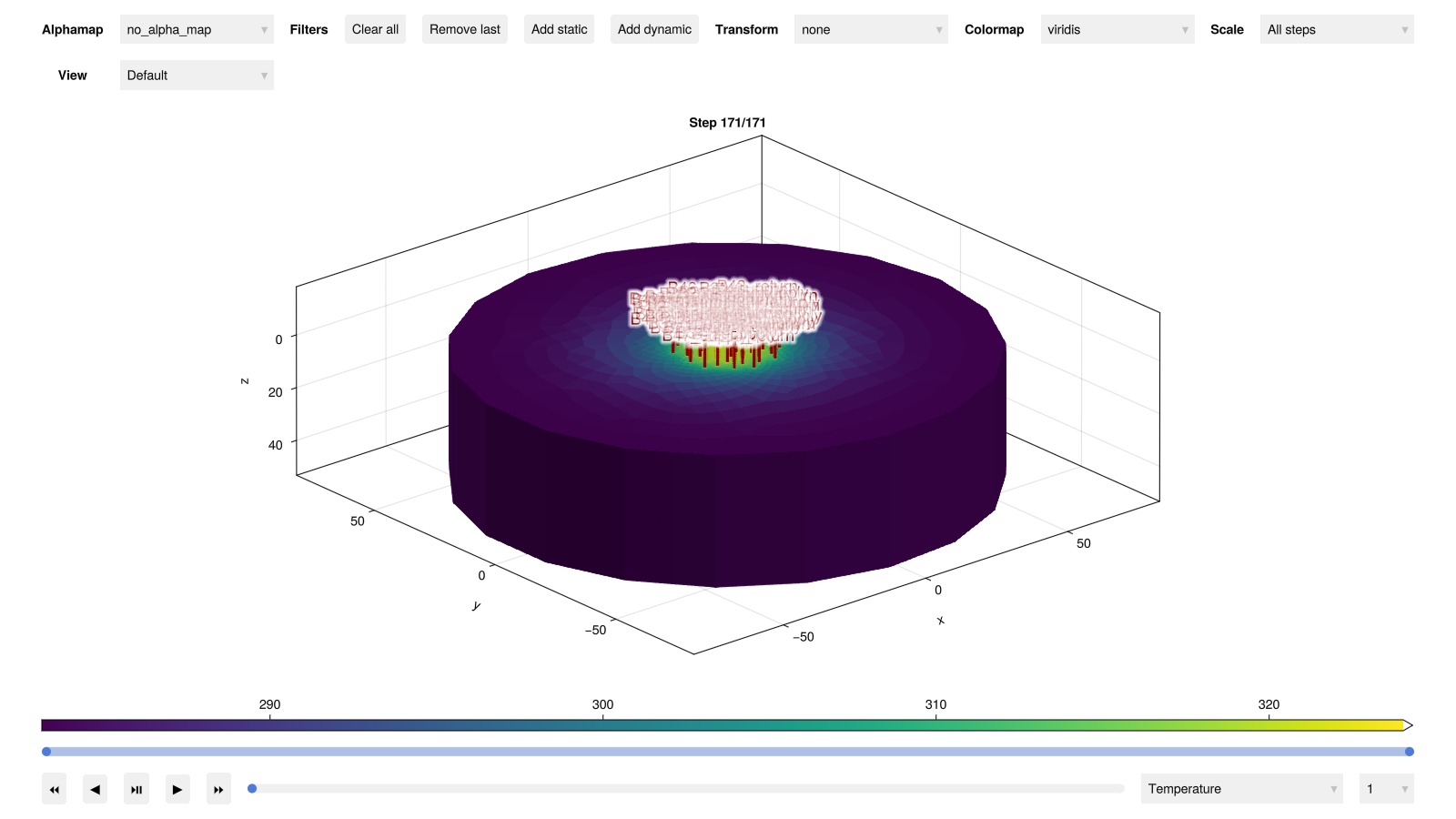
Inspect well solutions
Interactive plot:
plot_well_results(results.wells, field = :temperature)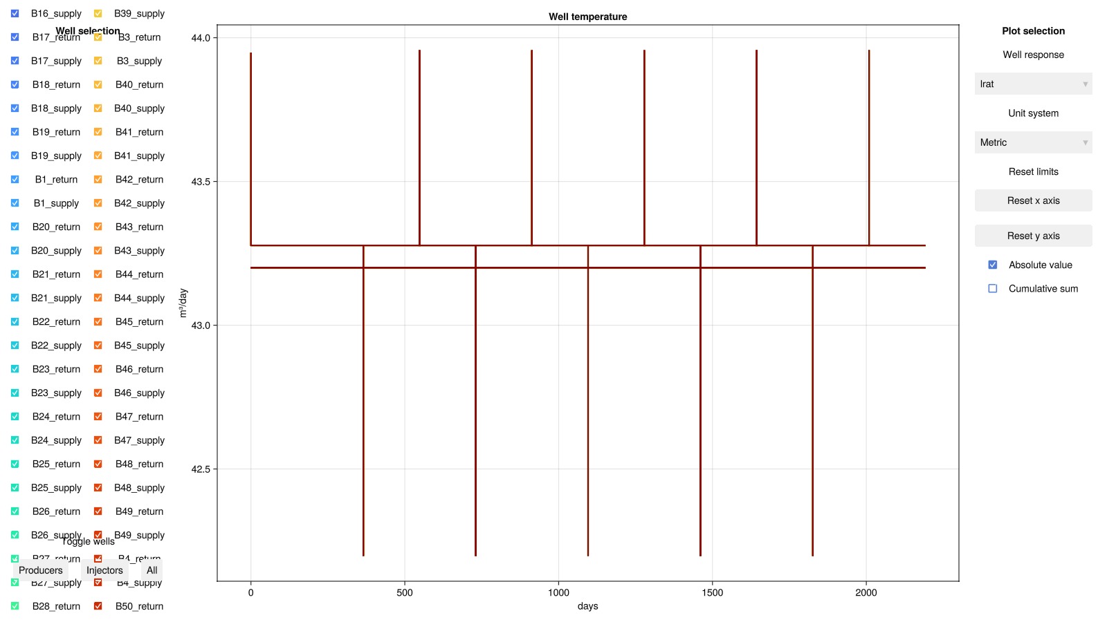
Return temperatures of center well vs time
temp = convert_from_si.(results.wells[:B1_return][:temperature], :Celsius)
time = cumsum(case.dt)/month
fig = Figure()
ax = Axis(fig[1, 1], title = "Center BTES temperature", xlabel = "Time (months)")
lines!(ax, time, temp)
fig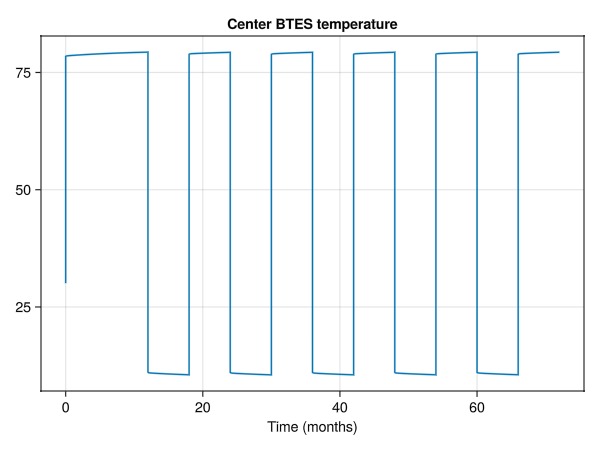
Example on GitHub
If you would like to run this example yourself, it can be downloaded from the JutulDarcy.jl GitHub repository as a script, or as a Jupyter Notebook
This example took 212.943642837 seconds to complete.This page was generated using Literate.jl.