Adding new wells to an existing model
Wells Advanced InputFile BlackoilTaking an existing reservoir model and modifying it with new wells is a typical operation in reservoir simulation. This example demonstrates how to add new wells to an existing model and a few ways to setup these wells.
The example uses the SPE1 data set as the model. We load the dataset as a JutulCase as usual and unpack the parts of the problem from the case before simulating the base case.
using Jutul, JutulDarcy, GLMakie
spe1_pth = JutulDarcy.GeoEnergyIO.test_input_file_path("SPE1", "SPE1.DATA")
case = setup_case_from_data_file(spe1_pth)
(; model, state0, forces, parameters, dt) = case
ws, states = simulate_reservoir(case)
ReservoirSimResult with 120 entries:
wells (2 present):
:INJ
:PROD
Results per well:
:wrat => Vector{Float64} of size (120,)
:Aqueous_mass_rate => Vector{Float64} of size (120,)
:orat => Vector{Float64} of size (120,)
:bhp => Vector{Float64} of size (120,)
:mrat => Vector{Float64} of size (120,)
:gor => Vector{Float64} of size (120,)
:lrat => Vector{Float64} of size (120,)
:mass_rate => Vector{Float64} of size (120,)
:rate => Vector{Float64} of size (120,)
:Vapor_mass_rate => Vector{Float64} of size (120,)
:control => Vector{Symbol} of size (120,)
:Liquid_mass_rate => Vector{Float64} of size (120,)
:wcut => Vector{Float64} of size (120,)
:grat => Vector{Float64} of size (120,)
states (Vector with 120 entries, reservoir variables for each state)
:Pressure => Vector{Float64} of size (300,)
:ImmiscibleSaturation => Vector{Float64} of size (300,)
:BlackOilUnknown => Vector{BlackOilX{Float64}} of size (300,)
:TotalMasses => Matrix{Float64} of size (3, 300)
:Rs => Vector{Float64} of size (300,)
:Saturations => Matrix{Float64} of size (3, 300)
time (report time for each state)
Vector{Float64} of length 120
result (extended states, reports)
SimResult with 120 entries
extra
Dict{Any, Any} with keys :simulator, :config
Completed at Jul. 10 2026 15:14 after 800 milliseconds, 697 microseconds, 248 nanoseconds.Replacing the existing wells with new wells with the same name
The simplest way to replace a well is to create a new well with the same name so that the new well replaces the old one. This is done by calling the setup routines and using the same name as the original wells. We place one injector and one producer, using the same names as in the original version of the case.
Here, we make use of the setup_well function to create the new wells and use the cell indices directly.
reservoir = reservoir_domain(model)
I1 = setup_well(reservoir, 1, name = :INJ)
P1 = setup_well(reservoir, 10, name = :PROD)
DataDomain wrapping SimpleWell [PROD] (1 nodes, 0 segments, 1 perforations) with 21 data fields added:
1 Perforations
:Kh => 1 Vector{Float64}
:skin => 1 Vector{Float64}
:perforation_radius => 1 Vector{Float64}
:well_index => 1 Vector{Float64}
:perforation_centroids => 3×1 Matrix{Float64}
:drainage_radius => 1 Vector{Float64}
:perforation_direction => 1 Vector{Symbol}
:cell_dims => 1 Vector{Tuple{Float64, Float64, Float64}}
:thermal_well_index => 1 Vector{Float64}
:net_to_gross => 1 Vector{Float64}
:permeability => 3×1 Matrix{Float64}
:thermal_conductivity => 1 Vector{Float64}
1 Cells
:cell_length => 1 Vector{Float64}
:radius => 1 Vector{Float64}
:radius_inner => 1 Vector{Float64}
:cell_centroids => 3×1 Matrix{Float64}
:volume_multiplier => 1 Vector{Float64}
:casing_thickness => 1 Vector{Float64}
:grouting_thickness => 1 Vector{Float64}
:casing_thermal_conductivity => 1 Vector{Float64}
:grouting_thermal_conductivity => 1 Vector{Float64}Add a new producer as multisegment well
We can also add more wells than originally present by adding new wells with new names. Some care will have to be taken later on to ensure that these wells have valid control and limits. We pick a cell with a IJK index to place this producer.
P2 = setup_well(reservoir, (10, 10, 1), name = :PROD_NEW, simple_well = false)DataDomain wrapping MultiSegmentWell [PROD_NEW] (1 nodes, 0 segments, 1 perforations) with 25 data fields added:
1 Perforations
:Kh => 1 Vector{Float64}
:skin => 1 Vector{Float64}
:perforation_radius => 1 Vector{Float64}
:well_index => 1 Vector{Float64}
:perforation_centroids => 3×1 Matrix{Float64}
:drainage_radius => 1 Vector{Float64}
:perforation_direction => 1 Vector{Symbol}
:cell_dims => 1 Vector{Tuple{Float64, Float64, Float64}}
:thermal_well_index => 1 Vector{Float64}
:net_to_gross => 1 Vector{Float64}
:permeability => 3×1 Matrix{Float64}
:thermal_conductivity => 1 Vector{Float64}
1 Cells
:cell_length => 1 Vector{Float64}
:radius => 1 Vector{Float64}
:radius_inner => 1 Vector{Float64}
:cell_centroids => 3×1 Matrix{Float64}
:volume_multiplier => 1 Vector{Float64}
:casing_thickness => 1 Vector{Float64}
:grouting_thickness => 1 Vector{Float64}
:casing_thermal_conductivity => 1 Vector{Float64}
:grouting_thermal_conductivity => 1 Vector{Float64}
:material_density => 1 Vector{Float64}
:material_heat_capacity => 1 Vector{Float64}
0 Faces
:roughness => 0 Vector{Float64}
:material_thermal_conductivity => 0 Vector{Float64}Add a new injector with a trajectory
An alternative to placing wells by cell index is to place them by trajectory. We can define a trajectory as a set of points in 3D space, here represented as a Matrix with three columns where each row represents a point along the trajectory. The trajectory is then used to discretize the well into cells.
traj = [
    50.0 3100.0 2500.0;
    56.0 2850.0 2540.0;
    120.0 2680.0 2550.0;
    400.0 2600.0 2565.0
]
I2 = setup_well_from_trajectory(reservoir, traj, name = :INJ_NEW)
DataDomain wrapping SimpleWell [INJ_NEW] (1 nodes, 0 segments, 5 perforations) with 21 data fields added:
5 Perforations
:Kh => 5 Vector{Float64}
:skin => 5 Vector{Float64}
:perforation_radius => 5 Vector{Float64}
:well_index => 5 Vector{Float64}
:perforation_centroids => 3×5 Matrix{Float64}
:drainage_radius => 5 Vector{Float64}
:perforation_direction => 5 Vector{Vector{Float64}}
:cell_dims => 5 Vector{Tuple{Float64, Float64, Float64}}
:thermal_well_index => 5 Vector{Float64}
:net_to_gross => 5 Vector{Float64}
:permeability => 3×5 Matrix{Float64}
:thermal_conductivity => 5 Vector{Float64}
1 Cells
:cell_length => 1 Vector{Float64}
:radius => 1 Vector{Float64}
:radius_inner => 1 Vector{Float64}
:cell_centroids => 3×1 Matrix{Float64}
:volume_multiplier => 1 Vector{Float64}
:casing_thickness => 1 Vector{Float64}
:grouting_thickness => 1 Vector{Float64}
:casing_thermal_conductivity => 1 Vector{Float64}
:grouting_thermal_conductivity => 1 Vector{Float64}Set up the new model
The new model is set up by calling the setup_reservoir_model function with the old model as the template. This function will create a new model with the same properties and customizations as the original model, but with the new wells added. The template model takes the place of the sys argument seen in other examples.
new_model = setup_reservoir_model(reservoir, model, wells = [I1, I2, P1, P2]);Visualize the new wells and the trajectory
We can see the new wells and the trajectory by plotting the model. Note that the trajectory is connected to cell centers in the numerical model. The coarse resolution of the model makes the trajectory appear jagged when realized along cells.
fig, ax, plt = plot_mesh_edges(reservoir)
lines!(ax, traj', color = :red)
for w in [I1, I2, P1, P2]
    plot_well!(ax, reservoir, w)
end
fig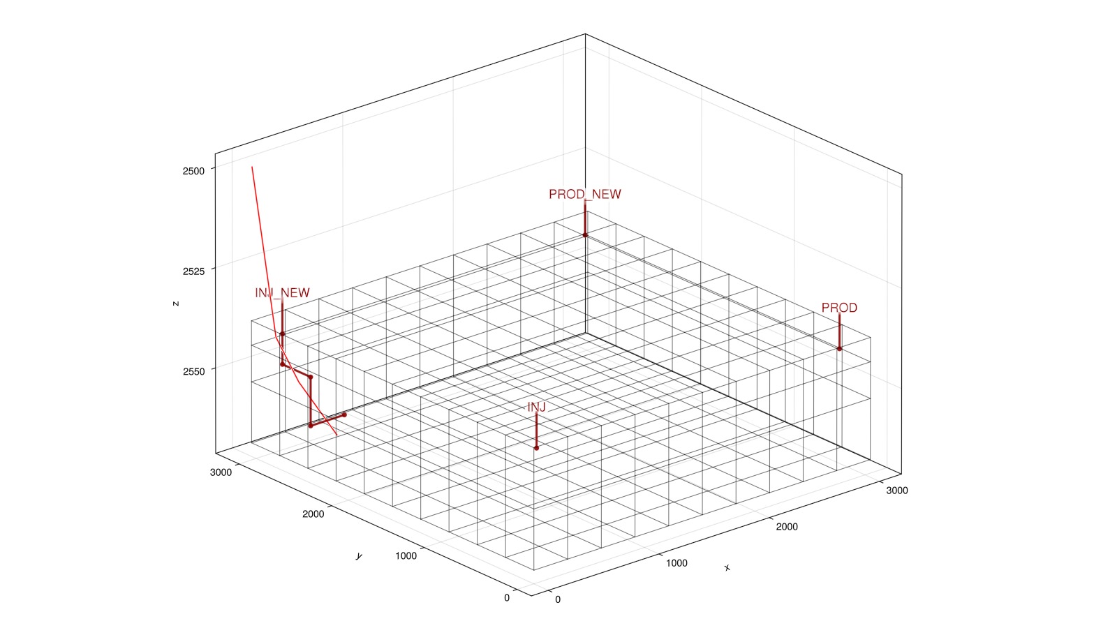
Setup a new state and forces
The new state and forces are set up in the same way as the original model, using the previous state0 and forces as templates. The new control and limits are duplicated from the old ones, mapping producer controls and limits to producers and injector controls and limits to injectors.
We keep the controls of the wells constant throughout the simulation, but we could also have made a forces Vector with one value per step.
new_state0 = setup_reservoir_state(new_model, state0)

new_control = Dict()
new_limits = Dict()

facility_forces = forces[1][:Facility]

ictrl = facility_forces.control[:INJ]
ilims = facility_forces.limits[:INJ]

pctrl = facility_forces.control[:PROD]
plims = facility_forces.limits[:PROD]

new_control[:INJ] = ictrl
new_control[:PROD] = pctrl
new_limits[:INJ] = ilims
new_limits[:PROD] = plims

new_control[:INJ_NEW] = ictrl
new_limits[:INJ_NEW] = ilims

new_control[:PROD_NEW] = pctrl
new_limits[:PROD_NEW] = plims

new_forces = setup_reservoir_forces(new_model, control = new_control, limits = new_limits)
Dict{Symbol, Any} with 6 entries:
:INJ => (mask = nothing,)
:PROD => (mask = nothing,)
:PROD_NEW => (mask = nothing,)
:Reservoir => (bc = nothing, sources = nothing)
:Facility => (control = Dict{Any, Any}(:INJ=>InjectorControl{TotalRateTarget…
:INJ_NEW => (mask = nothing,)Simulate the new case
new_ws, new_states = simulate_reservoir(new_state0, new_model, dt, forces = new_forces)ReservoirSimResult with 120 entries:
wells (4 present):
:INJ
:PROD
:PROD_NEW
:INJ_NEW
Results per well:
:wrat => Vector{Float64} of size (120,)
:Aqueous_mass_rate => Vector{Float64} of size (120,)
:orat => Vector{Float64} of size (120,)
:bhp => Vector{Float64} of size (120,)
:mrat => Vector{Float64} of size (120,)
:gor => Vector{Float64} of size (120,)
:lrat => Vector{Float64} of size (120,)
:mass_rate => Vector{Float64} of size (120,)
:rate => Vector{Float64} of size (120,)
:Vapor_mass_rate => Vector{Float64} of size (120,)
:control => Vector{Symbol} of size (120,)
:Liquid_mass_rate => Vector{Float64} of size (120,)
:wcut => Vector{Float64} of size (120,)
:grat => Vector{Float64} of size (120,)
states (Vector with 120 entries, reservoir variables for each state)
:Pressure => Vector{Float64} of size (300,)
:ImmiscibleSaturation => Vector{Float64} of size (300,)
:BlackOilUnknown => Vector{BlackOilX{Float64}} of size (300,)
:TotalMasses => Matrix{Float64} of size (3, 300)
:Rs => Vector{Float64} of size (300,)
:Saturations => Matrix{Float64} of size (3, 300)
time (report time for each state)
Vector{Float64} of length 120
result (extended states, reports)
SimResult with 120 entries
extra
Dict{Any, Any} with keys :simulator, :config
Completed at Jul. 10 2026 15:14 after 9 seconds, 485 milliseconds, 167.4 microseconds.Visualize the results
We can visualize the results of the new model and the old model
plot_reservoir(new_model, new_states, title = "New wells", step = 120, key = :Rs)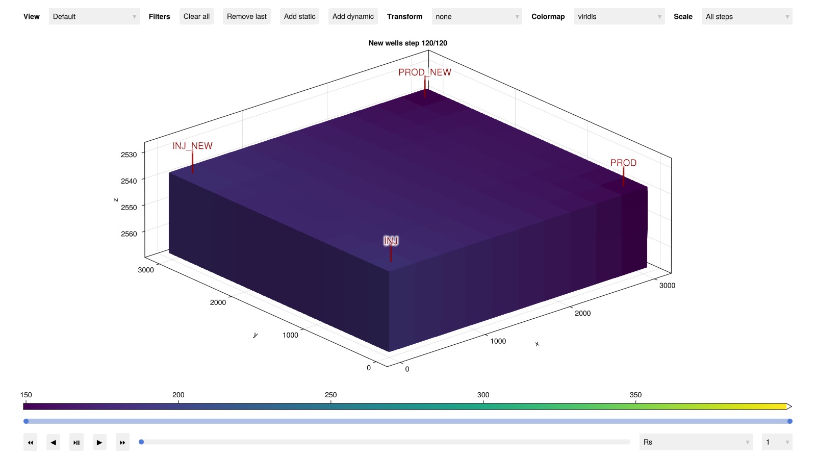
We can also visualize the original model for comparison
plot_reservoir(model, states, title = "Original wells", step = 120, key = :Pressure)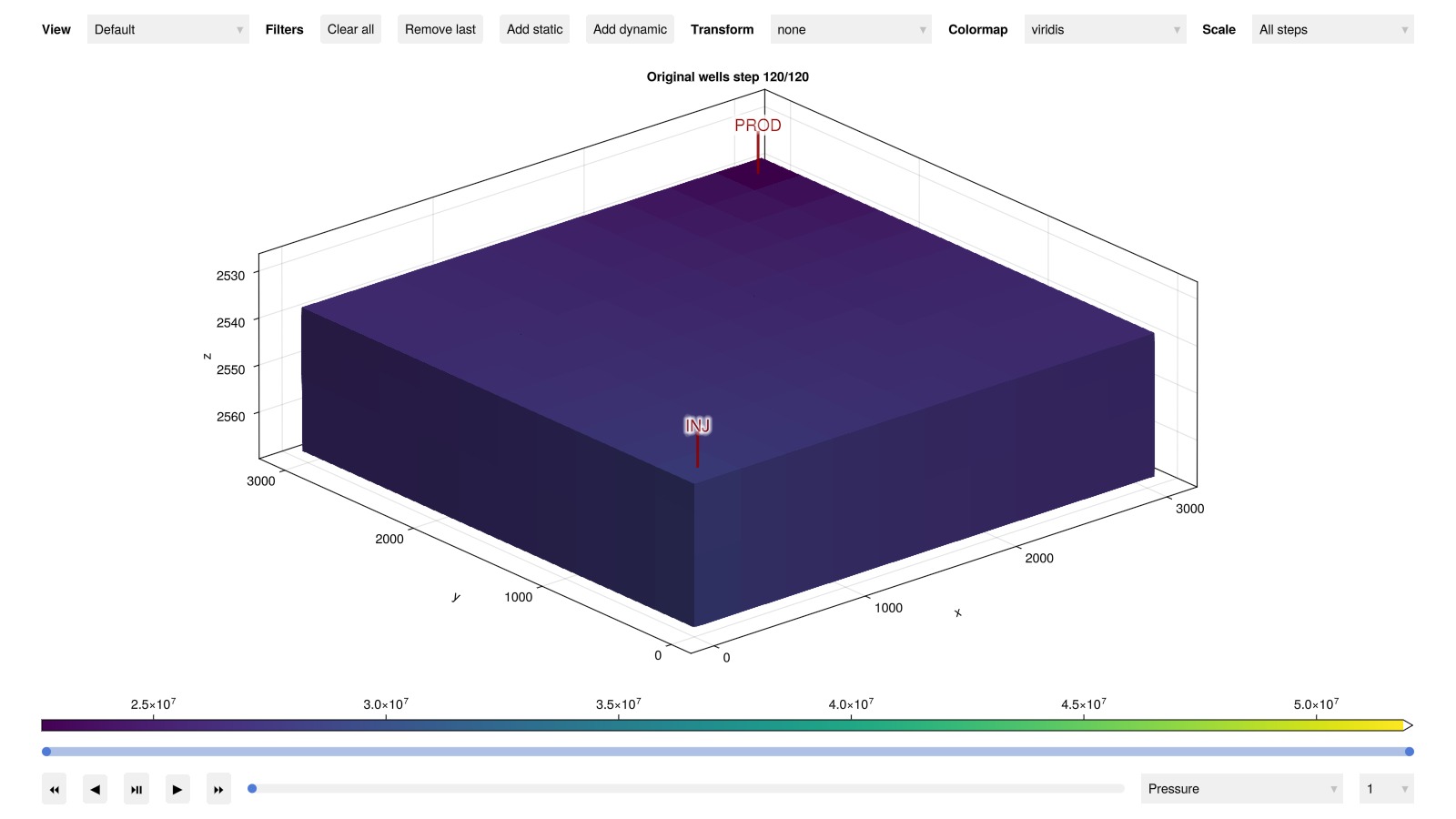
Side by side comparison
g = physical_representation(reservoir)
fig = Figure(size = (1200, 600))
ax = Axis3(fig[1, 1], zreversed = true, title = "Original wells")
plt = plot_cell_data!(ax, g, states[120][:Saturations][3, :], colorrange = (0.0, 0.7))
ax = Axis3(fig[1, 2], zreversed = true, title = "New wells")
plot_cell_data!(ax, g, new_states[120][:Saturations][3, :], colorrange = (0.0, 0.7))
Colorbar(fig[1, 3], plt)
fig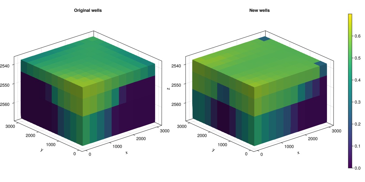
Example on GitHub
If you would like to run this example yourself, it can be downloaded from the JutulDarcy.jl GitHub repository as a script
This example took 41.978018215 seconds to complete.This page was generated using Literate.jl.