Model coarsening

Running a model at full resolution can be computationally expensive. In many cases, it is possible to coarsen the model to reduce the computational cost. This example demonstrates how to coarsen a model using JutulDarcy.jl. The example uses the Egg model, which is a small oil-water model with heterogeneous permeability. The model is coarsened using different methods and partition sizes, and the results are compared to the fine-scale model. The example demonstrates how to coarsen a model and simulate it using JutulDarcy.jl. The example also demonstrates how to compare the results of the coarse-scale model to the fine-scale model.

The example is intended to show the workflow of coarsening a model, and represents a starting point for more advanced techniques like upscaling, coarse-model calibration and history matching. The model is therefore intentionally simple and very coarse for quick simulations, and not necessarily accurate model responses.

using Jutul, JutulDarcy, HYPRE
using GLMakie
using GeoEnergyIO
data_dir = GeoEnergyIO.test_input_file_path("EGG")
data_pth = joinpath(data_dir, "EGG.DATA")
fine_case = setup_case_from_data_file(data_pth);

Simulate the base case

We simulate the fine case to get a reference solution to compare against. We also extract the mesh and reservoir for plotting.

fine_model = fine_case.model
fine_reservoir = reservoir_domain(fine_model)
fine_mesh = physical_representation(fine_reservoir)
ws, states = simulate_reservoir(fine_case, info_level = -1);

Coarsen the model and plot partition

We coarsen the model using a partition size of 20x20x2 and the IJK method where the underlying structure of the mesh is used to subdivide the blocks. This function automatically handles inactive cells and disconnected blocks and can therefore also work on more complex models.

We pass a triplet of integers to specify the partition size. This will give an essentially structured partition. Later on, we we will look at graph partitioners.

coarse_case = coarsen_reservoir_case(fine_case, (20, 20, 2), method = :ijk)
coarse_model = coarse_case.model
coarse_reservoir = reservoir_domain(coarse_case)
coarse_mesh = physical_representation(coarse_reservoir)

p = coarse_mesh.partition

fig, = plot_cell_data(fine_mesh, p, colormap = :lipariS)
fig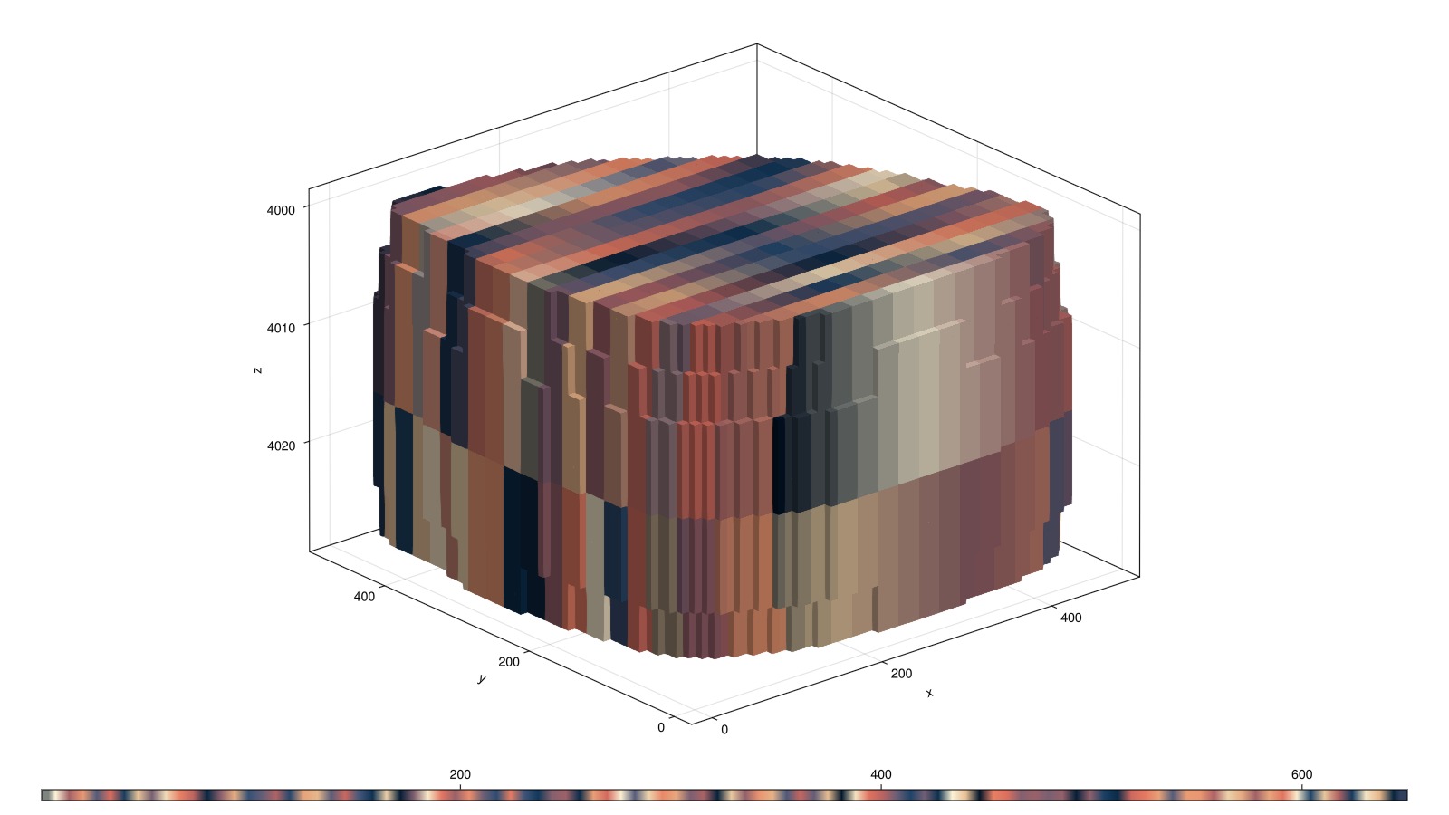

Compare fine-scale and coarse-scale permeability

The fine-scale and coarse-scale permeability fields are compared visually. The coarsening uses a static upscaling, where the permeability is harmonically averaged per direction when coarsening. This is a simple method that can be effective enough for many cases.

The fine-scale permeability is shown on the left, and the coarse-scale is shown on the right, with the same color axis.

K_f = fine_reservoir[:permeability][1, :]
K_c = coarse_reservoir[:permeability][1, :]

kcaxis = extrema(K_f)

fig = Figure(size = (1200, 500))
axf = Axis3(fig[1, 1], title = "Fine scale permeability", zreversed = true)
plot_cell_data!(axf, fine_mesh, K_f, colorrange = kcaxis, colormap = :turbo)

axc = Axis3(fig[1, 2], title = "Coarse scale permeability", zreversed = true)
plt = plot_cell_data!(axc, coarse_mesh, K_c, colorrange = kcaxis, colormap = :turbo)
Colorbar(fig[1, 3], plt)
fig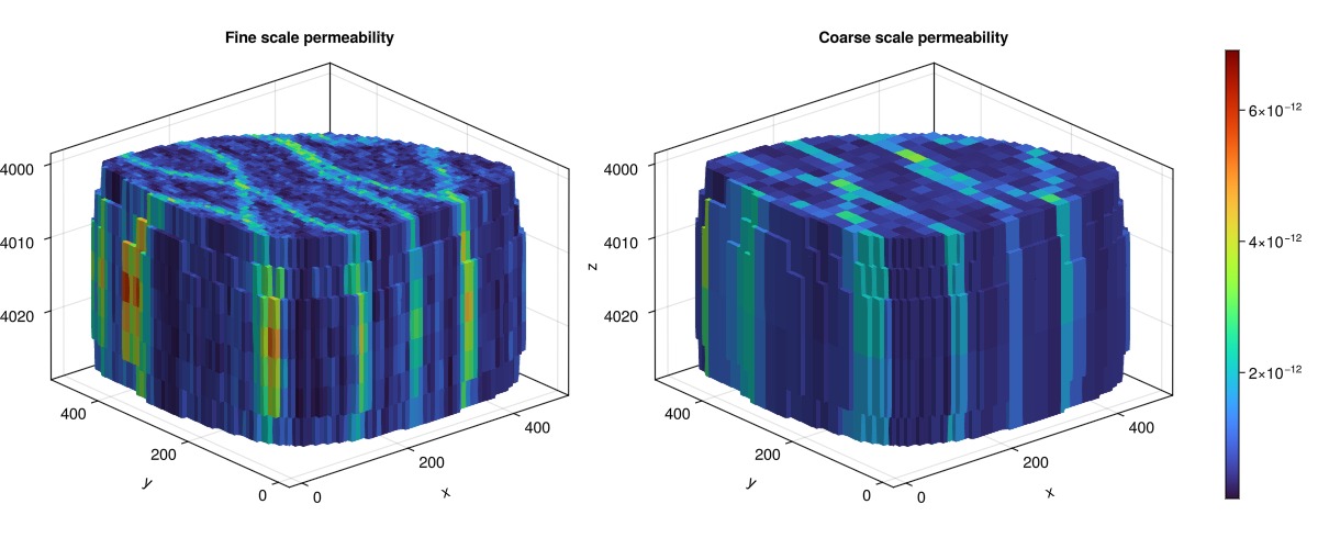

Simulate the coarse-scale model

The coarse scale model can be simulated just as the fine-scale model was, but the runtime should be significantly reduced down to around a second.

@time ws_c, states_c = simulate_reservoir(coarse_case, info_level = -1);

  1.118194 seconds (3.76 M allocations: 314.147 MiB, 3.91% gc time, 3.51% compilation time: 100% of which was recompilation)

Plot and compare the coarse-scale and fine-scale solutions

We plot the pressure field for the fine-scale and coarse-scale models. The model has little pressure variation, but we see that there are substantial differences between our very coarse model and the original fine-scale.

using Statistics
wells = JutulDarcy.get_model_wells(fine_model)

p_c = states_c[end][:Pressure]
p_f = states[end][:Pressure]

caxis = extrema([extrema(p_c)..., extrema(p_f)...])

fig = Figure(size = (1200, 500))
axf = Axis3(fig[1, 1], title = "Fine scale", zreversed = true)
plot_cell_data!(axf, fine_mesh, p_f, colorrange = caxis, colormap = :turbo)

for (k, w) in wells
    plot_well!(axf, fine_mesh, w, fontsize = 0)
end

axc = Axis3(fig[1, 2], title = "Coarse scale", zreversed = true)
plt = plot_cell_data!(axc, coarse_mesh, p_c, colorrange = caxis, colormap = :turbo)

for (k, w) in wells
    plot_well!(axc, fine_mesh, w, fontsize = 0)
end
Colorbar(fig[1, 3], plt)
fig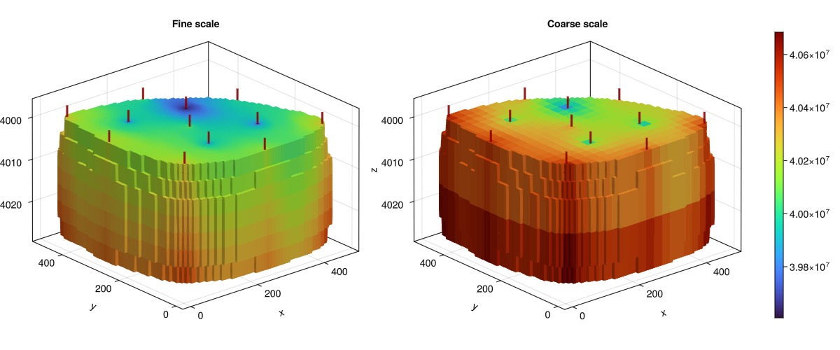

Plot and compare the saturation fields

We observe that the saturation fields are quite different between the coarse-scale and fine scale, with the coarse-scale model showing a more uniform saturation field as the leading shock is smeared away.

s_c = states_c[end][:Saturations][1, :]
s_f = states[end][:Saturations][1, :]

scaxis = extrema([extrema(s_c)..., extrema(s_f)...])

fig = Figure(size = (1200, 500))
axf = Axis3(fig[1, 1], title = "Fine scale", zreversed = true)
plot_cell_data!(axf, fine_mesh, s_f, colorrange = scaxis, colormap = :turbo)

for (k, w) in wells
    plot_well!(axf, fine_mesh, w, fontsize = 0)
end

axc = Axis3(fig[1, 2], title = "Coarse scale", zreversed = true)
plt = plot_cell_data!(axc, coarse_mesh, s_c, colorrange = scaxis, colormap = :turbo)

for (k, w) in wells
    plot_well!(axc, fine_mesh, w, fontsize = 0)
end
Colorbar(fig[1, 3], plt)
fig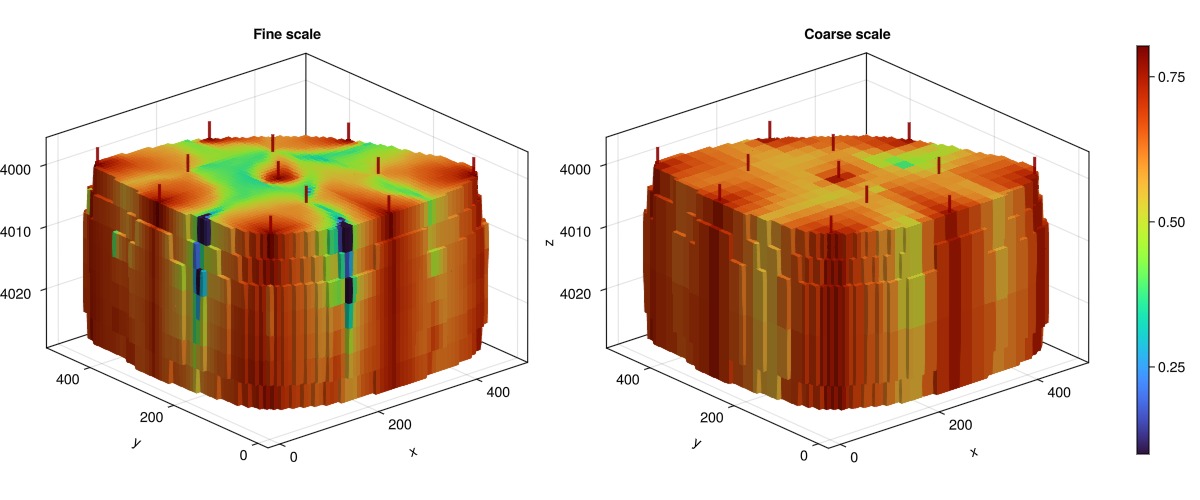

Plot the average field scale pressure evolution

fig = Figure()
axf_p = Axis(fig[1, 1], ylabel = "Avg. pressure / bar")
lines!(axf_p, map(x -> mean(x[:Pressure])/1e5, states), label = "Fine")
lines!(axf_p, map(x -> mean(x[:Pressure])/1e5, states_c), label = "Coarse")
axislegend()
fig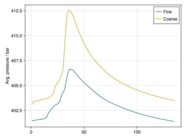

Plot the wells interactively

We can plot the well results in the interactive viewer using the comparison feature that allows multiple results to be superimposed in the same figure.

plot_well_results([ws, ws_c], names = ["Fine", "Coarse"], field = :orat, accumulated = true)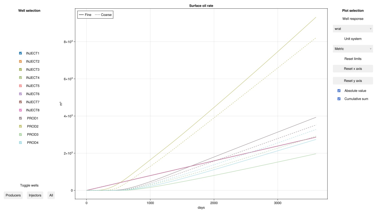

Plot field scale measurables over time interactively

The field-scale quantities match fairly well between the coarse-scale and fine-scale models. There is always a trade-off between accuracy and quality in numerical simulations, where the goal is to find the right balance between accuracy in quantities of interest and computational cost.

fine_m = reservoir_measurables(fine_case, ws, states)
coarse_m = reservoir_measurables(coarse_case, ws_c, states_c)
m = copy(fine_m)
for (k, v) in pairs(coarse_m)
    if k != :time
        m[Symbol("coarse_$k")] = v
    end
end

plot_reservoir_measurables(m, left = :fopr, right = :coarse_fopr, accumulated = true)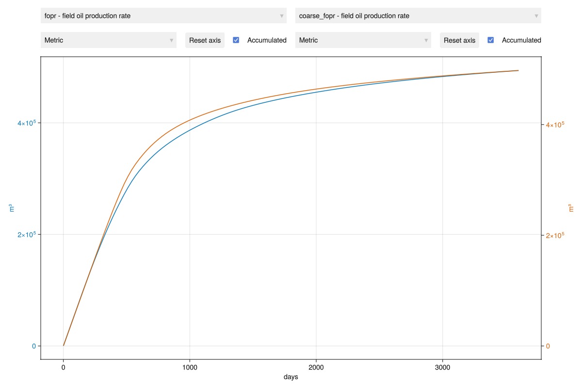

Compare different partitioning methods

We have only so far tested a single partitioning method. We can quickly generate a few other coarse models using different partitioning methods and coarsening values. We highlight that we can also use the centroids instead of the IJK indices to partition, for when the mesh may not have a structured background mesh. In addition, we can call different graph partitioners by passing the desired number of blocks. Here, we call a simple METIS-based transmissibility coarsening, but the code contains options to use other weights and partitioners.

partition_variants = [
    (:centroids, (3, 3, 2)),
    (:ijk, (5, 5, 1)),
    (:metis, 10),
    (:metis, 50)
]

fig = Figure(size = (1200, 600))
layout = GridLayout()
fig[1, 1] = layout
rowwidth = Int(floor(length(partition_variants)/2))
for (no, variant) in enumerate(partition_variants)
    if no > rowwidth
        row = 2
        pix = no - rowwidth
    else
        row = 1
        pix = no
    end
    cmethod, cdim = variant
    variant_case = coarsen_reservoir_case(fine_case, cdim, method = cmethod)
    r = reservoir_domain(variant_case)
    m = physical_representation(r)
    p = m.partition

    ax = Axis3(fig, title = "$cmethod - $cdim", azimuth = 0.3, elevation = 1.0, zreversed = true)
    plot_cell_data!(ax, fine_mesh, p, colormap = :lipariS)
    layout[row, 2*(pix-1) + 1] = ax

    _, variant_states = simulate_reservoir(variant_case, info_level = -1)
    pres = variant_states[end][:Pressure]
    axp = Axis3(fig, title = "Pressure", azimuth = 0.3, elevation = 1.0, zreversed = true)
    for (k, w) in wells
        plot_well!(axp, fine_mesh, w, fontsize = 0)
    end
    plot_cell_data!(axp, m, pres, colorrange = caxis, colormap = :turbo)

    layout[row, 2*(pix-1) + 2] = axp
end
fig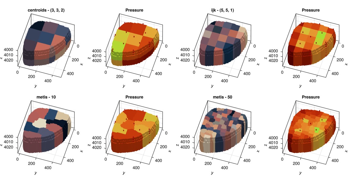

Example on GitHub

If you would like to run this example yourself, it can be downloaded from the JutulDarcy.jl GitHub repository as a script, or as a Jupyter Notebook

This example took 54.347172281 seconds to complete.

---

This page was generated using Literate.jl.