Simulating Eclipse/DATA input files
Introduction InputFileThe DATA format is commonly used in reservoir simulation. JutulDarcy can set up cases on this format and includes a fully featured grid builder for corner-point grids. Once a case has been set up, it uses the same types as a regular JutulDarcy simulation, allowing modification and use of the case in differentiable workflows.
We begin by loading the SPE9 dataset via the GeoEnergyIO package. This package includes a set of open datasets that can be used for testing and benchmarking. The SPE9 dataset is a 3D model with a corner-point grid and a set of wells produced by the Society of Petroleum Engineers. The specific version of the file included here is taken from the OPM tests repository.
using JutulDarcy, GeoEnergyIO
pth = GeoEnergyIO.test_input_file_path("SPE9", "SPE9.DATA");
Set up and run a simulation
We have supressed the output of the simulation to avoid cluttering the documentation, but we can set the info_level to a higher value to see the output.
If we do not need the case, we could also have simulated by passing the path: ws, states = simulate_data_file(pth)
case = setup_case_from_data_file(pth)
simulated = simulate_reservoir(case);
ws, states = simulated;
PVT: Fixing table for low pressure conditions.
Jutul: Simulating 2 years, 24.22 weeks as 90 report steps
╭────────────────┬──────────┬──────────────┬──────────╮
│ Iteration type │ Avg/step │ Avg/ministep │ Total │
│ │ 90 steps │ 95 ministeps │ (wasted) │
├────────────────┼──────────┼──────────────┼──────────┤
│ Newton │ 3.55556 │ 3.36842 │ 320 (0) │
│ Linearization │ 4.61111 │ 4.36842 │ 415 (0) │
│ Linear solver │ 11.3889 │ 10.7895 │ 1025 (0) │
│ Precond apply │ 22.7778 │ 21.5789 │ 2050 (0) │
╰────────────────┴──────────┴──────────────┴──────────╯
╭───────────────┬─────────┬────────────┬─────────╮
│ Timing type │ Each │ Relative │ Total │
│ │ ms │ Percentage │ s │
├───────────────┼─────────┼────────────┼─────────┤
│ Properties │ 2.7699 │ 5.59 % │ 0.8864 │
│ Equations │ 6.4101 │ 16.79 % │ 2.6602 │
│ Assembly │ 2.9508 │ 7.73 % │ 1.2246 │
│ Linear solve │ 2.3574 │ 4.76 % │ 0.7544 │
│ Linear setup │ 12.9572 │ 26.17 % │ 4.1463 │
│ Precond apply │ 1.0142 │ 13.12 % │ 2.0792 │
│ Update │ 1.6836 │ 3.40 % │ 0.5387 │
│ Convergence │ 2.5897 │ 6.78 % │ 1.0747 │
│ Input/Output │ 2.3123 │ 1.39 % │ 0.2197 │
│ Other │ 7.0639 │ 14.27 % │ 2.2604 │
├───────────────┼─────────┼────────────┼─────────┤
│ Total │ 49.5143 │ 100.00 % │ 15.8446 │
╰───────────────┴─────────┴────────────┴─────────╯Show the input data
The input data takes the form of a Dict:
case.input_dataDict{String, Any} with 6 entries:
"RUNSPEC" => OrderedDict{String, Any}("TITLE"=>"SPE 9", "DIMENS"=>[24, 25, 1…
"GRID" => OrderedDict{String, Any}("cartDims"=>(24, 25, 15), "CURRENT_BOX…
"PROPS" => OrderedDict{String, Any}("PVTW"=>Any[[2.48211e7, 1.0034, 4.3511…
"SUMMARY" => OrderedDict{String, Any}()
"SCHEDULE" => Dict{String, Any}("STEPS"=>OrderedDict{String, Any}[OrderedDict…
"SOLUTION" => OrderedDict{String, Any}("EQUIL"=>Any[[2753.87, 2.48211e7, 3032…We can also examine the for example RUNSPEC section, which is also represented as a Dict.
case.input_data["RUNSPEC"]OrderedDict{String, Any} with 13 entries:
"TITLE" => "SPE 9"
"DIMENS" => [24, 25, 15]
"OIL" => true
"WATER" => true
"GAS" => true
"DISGAS" => true
"FIELD" => true
"START" => DateTime("2015-01-01T00:00:00")
"WELLDIMS" => [26, 5, 1, 26, 5, 10, 5, 4, 3, 0, 1, 1, 10, 201]
"TABDIMS" => [1, 1, 40, 20, 1, 20, 20, 1, 1, -1 … -1, 10, 10, 10, -1, 5, 5…
"EQLDIMS" => [1, 100, 50, 1, 50]
"UNIFIN" => true
"UNIFOUT" => truePlot the simulation model
These plot are normally interactive, but if you are reading the published online documentation static screenshots will be inserted instead.
using GLMakie
plot_reservoir(case.model, states)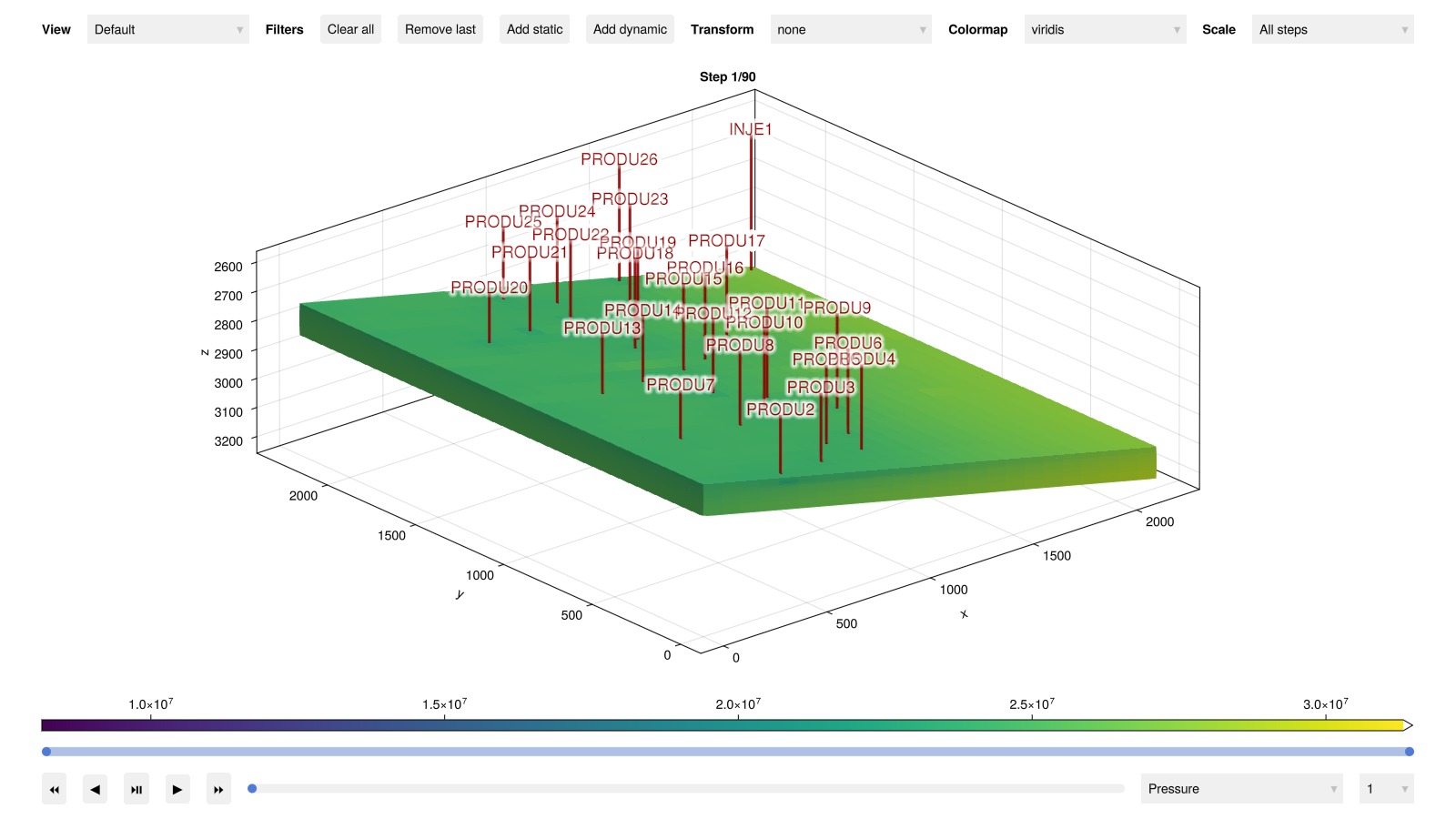
Plot the well responses
We can plot the well responses (rates and pressures) in an interactive viewer. Multiple wells can be plotted simultaneously, with options to select which units are to be used for plotting.
plot_well_results(ws)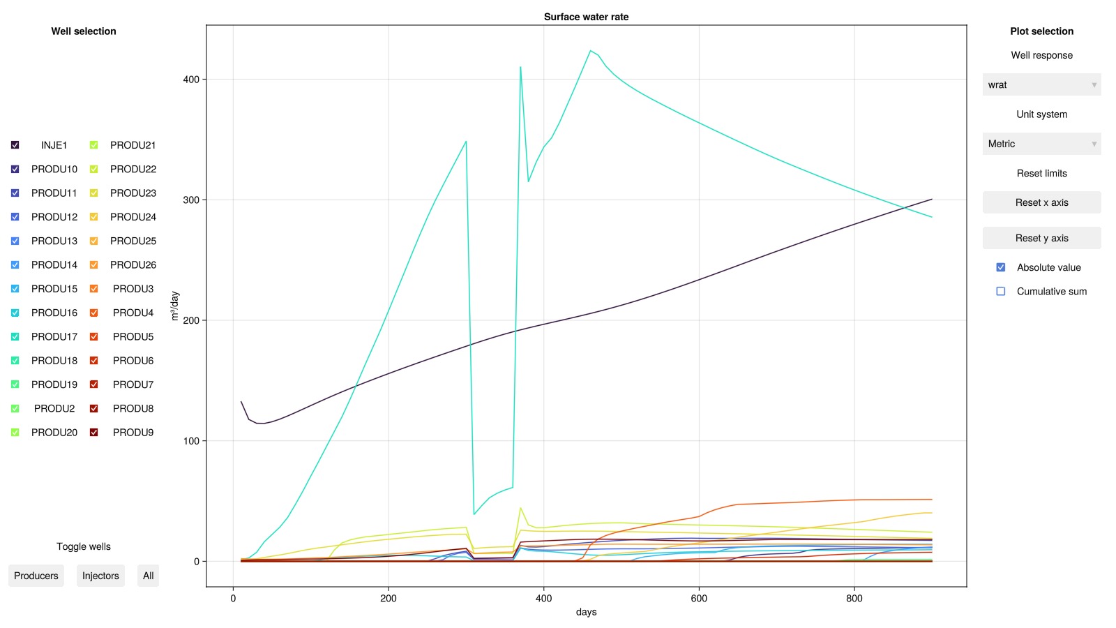
Plot the field responses
Similar to the wells, we can also plot field-wide measurables. We plot the field gas production rate and the average pressure as the initial selection. If you are running this case interactively you can select which measurables to plot.
We observe that the field pressure steadily decreases over time, as a result of the gas production. The drop in pressure is not uniform, as during the period where little gas is produced, the decrease in field pressure is slower.
plot_reservoir_measurables(case, ws, states, left = :fgpr, right = :pres)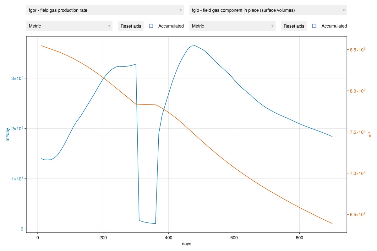
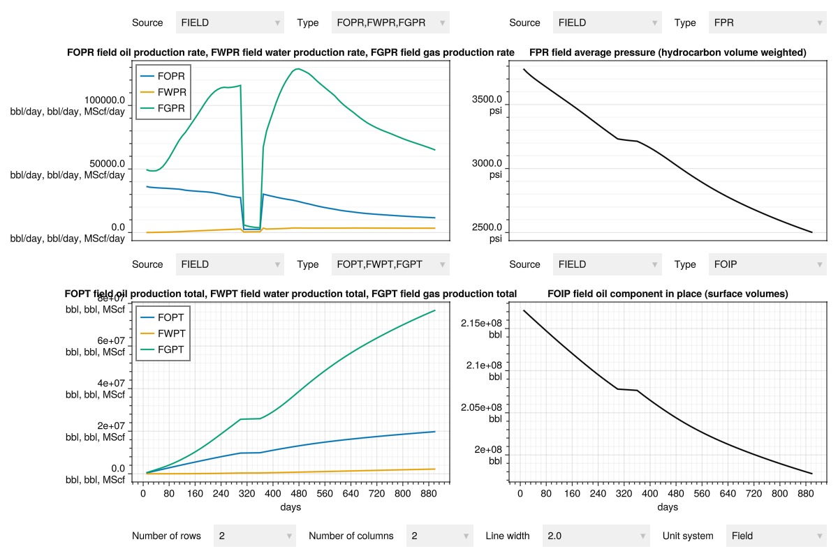
Plot the summary data
The summary contains field and well responses in one file. We have a dedicated viewer that can be preconfigured to show specific responses, or used interactively to explore.
JutulDarcy.plot_summary(simulated.summary)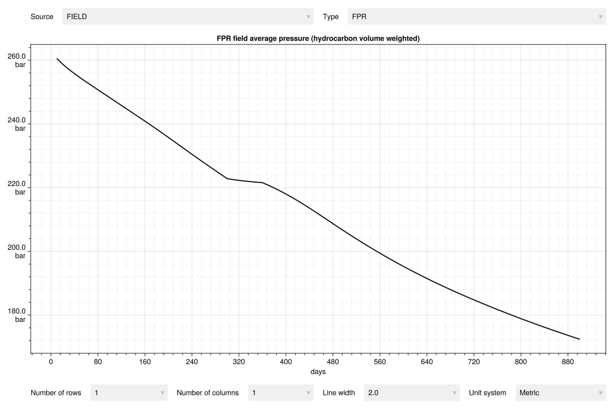
We can also pre-specify and group plot responses
JutulDarcy.plot_summary(simulated.summary,
    plots = ["FOPR,FWPR,FGPR", "FOPT,FWPT,FGPT", "FPR", "FOIP"],
    unit_system = "Field",
    cols = 2
)
Plot in free camera 3D viewer
The 3D viewer allows us to explore the grid and solution in more detail. The free camera allows for detailed inspection of the grid and is closer to typical reservoir simulation visualizers that the default plot_reservoir code.
using Jutul
reservoir = reservoir_domain(case)
ex = plot_explorer(reservoir, dynamic = simulated.states, colormap = :seaborn_icefire_gradient)
for (k, w) in get_model_wells(case.model)
    plot_well!(ex.lscene, reservoir, w)
end
ex.fig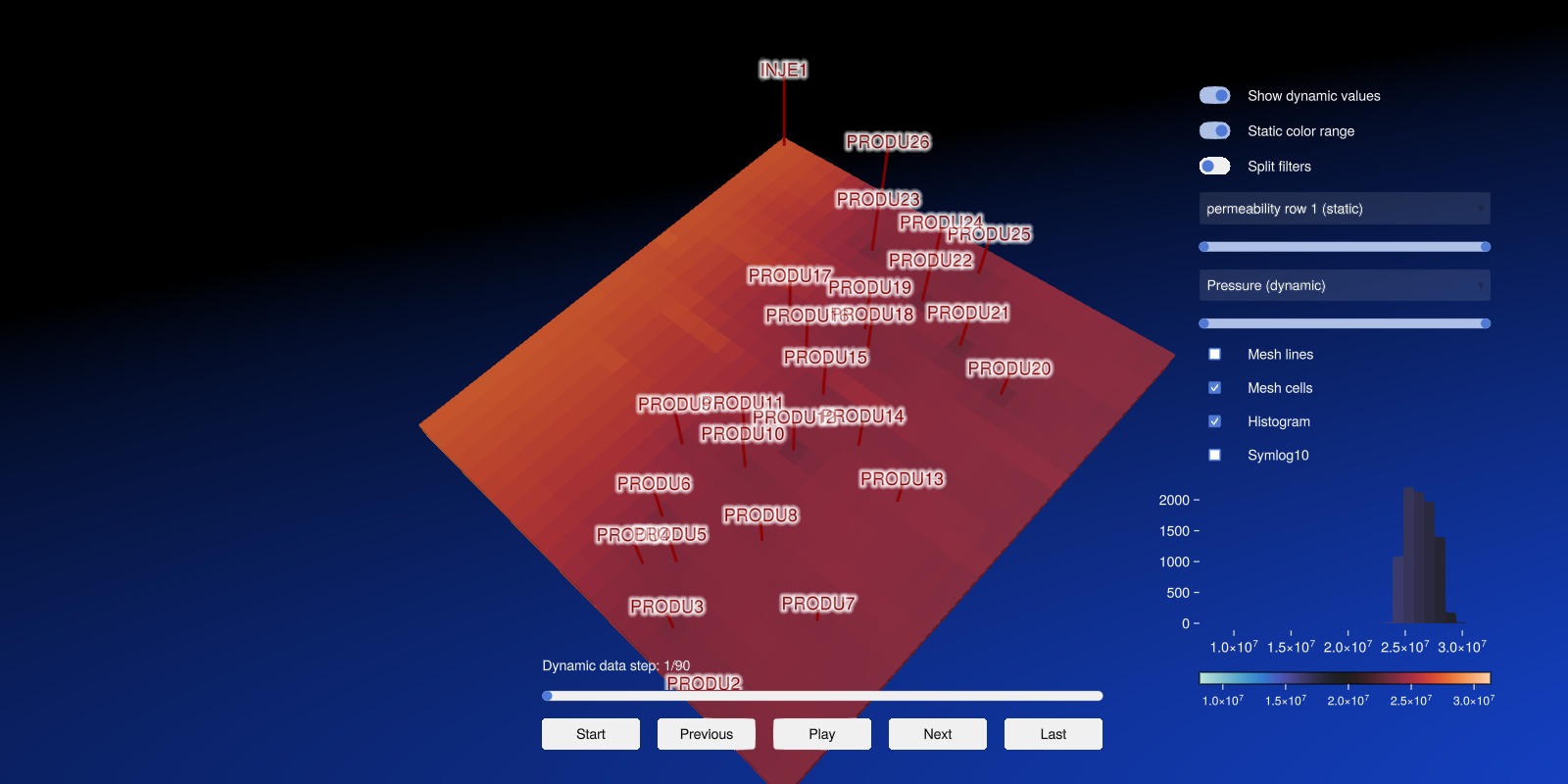
Example on GitHub
If you would like to run this example yourself, it can be downloaded from the JutulDarcy.jl GitHub repository as a script
This example took 49.982986332 seconds to complete.This page was generated using Literate.jl.