Consistent and high-resolution: WENO, NTPFA and AvgMPFA

The following example demonstrates how to set up a reservoir model with different discretizations for flow and transport for a skewed grid. The model setup is taken from 6.1.2 in the MRST book [1].

The example is a two-dimensional model with a single layer. The domain itself is completely symmetric, with producer in either lower corner and a single injector in the middle of the domain. From a flow perspective, the model is completely symmetric, and exactly the same results should be obtained for both producer wells. The grid is intentionally distorted to be skewed towards one producer, which will lead to consistency issues for the standard two-point flux approximation used by the solvers.

The fluid model is also quite simple, with two immiscible phases that have linear relative permeability functions. A consequence of this is that the fluid fronts are not self-sharpening and are expected to be smeared out due to the numerical diffusion of the standard first-point upwind scheme.

using Jutul, JutulDarcy, GLMakie
Darcy, kg, meter, day, bar = si_units(:darcy, :kg, :meter, :day, :bar)
ny = 20
nx = 2*ny + 1
nz = 1

gcart = CartesianMesh((nx, ny, nz), (2.0, 1.0, 1.0))
g = UnstructuredMesh(gcart)

for (i, pt) in enumerate(g.node_points)
    x, y, z = pt
    pt += [0.4*(1.0-(x-1.0)^2)*(1.0-y), 0, 0]
    g.node_points[i] = pt .* [1000.0, 1000.0, 1.0]
end

c_i = cell_index(g, (nx÷2+1, ny, 1))
c_p1 = cell_index(g, (1, 1, 1))
c_p2 = cell_index(g, (nx, 1, 1))

fig = Figure()
ax = Axis(fig[1, 1])
Jutul.plot_mesh_edges!(ax, g)
plot_mesh!(ax, g, cells = c_i, color = :red)
plot_mesh!(ax, g, cells = [c_p1, c_p2], color = :blue)
fig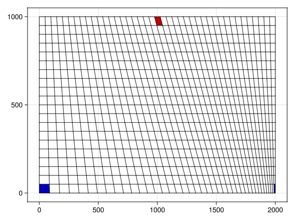

Define wells, fluid system and controls

reservoir = reservoir_domain(g, permeability = 0.1Darcy, porosity = 0.1)

c_i1 = cell_index(g, (nx÷2+1, ny, 1))

I1 = setup_vertical_well(reservoir, nx÷2+1, ny, name = :I1, simple_well = true)
P1 = setup_vertical_well(reservoir, 1, 1, name = :P1, simple_well = true)
P2 = setup_vertical_well(reservoir, nx, 1, name = :P2, simple_well = true)

phases = (AqueousPhase(), LiquidPhase())
rhoWS = rhoLS = 1000.0
rhoS = [rhoWS, rhoLS] .* kg/meter^3
sys = ImmiscibleSystem(phases, reference_densities = rhoS)

dt = repeat([30.0]*day, 100)
pv = pore_volume(reservoir)
inj_rate = sum(pv)/sum(dt)

rate_target = TotalRateTarget(inj_rate)
I_ctrl = InjectorControl(rate_target, [1.0, 0.0], density = rhoWS)
bhp_target = BottomHolePressureTarget(50*bar)
P_ctrl = ProducerControl(bhp_target)
controls = Dict()
controls[:I1] = I_ctrl
controls[:P1] = P_ctrl
controls[:P2] = P_ctrl

ProducerControl{BottomHolePressureTarget{Float64}, Float64}(BottomHolePressureTarget with value 50.0 [bar], 1.0)

Define functions to perform the simulations

We are going to perform a number of simulations with different discretizations and it is therefore convenient to setup functions that can be called with the desired discretizations as arguments. The results are stored in a dictionary for easy retrieval after the simulations are done.

all_results = Dict()

Dict{Any, Any}()

Function to perform simulation

The function simulate_with_discretizations sets up the reservoir model with the requested discretizations. The default behavior mirrors the default behavior of JutulDarcy by using the industry standard single-point upwind, two-point flux approximation.

function simulate_with_discretizations(upwind = :spu, kgrad = :tpfa)
    model, parameters = setup_reservoir_model(reservoir, sys,
        kgrad = kgrad,
        upwind = upwind,
        wells = [P1, P2, I1]
    )
    kr = BrooksCoreyRelativePermeabilities(sys, 1.0, 0.0, 1.0)
    replace_variables!(model, RelativePermeabilities = kr)
    forces = setup_reservoir_forces(model, control = controls)
    state0 = setup_reservoir_state(model, Pressure = 100*bar, Saturations = [0.0, 1.0])
    result = simulate_reservoir(state0, model, dt, info_level = 0, parameters = parameters, forces = forces);
end

simulate_with_discretizations (generic function with 3 methods)

Function to plot the results

We create a function plot_discretization_result that takes the result from a simultation and plots the saturation field after 75 steps.

function plot_discretization_result(result, name)
    ws, states = result
    sg = states[75][:Saturations][1, :]
    fig = Figure()
    ax = Axis(fig[1, 1], title = name)
    plot_cell_data!(ax, g, sg, colormap = :seaborn_icefire_gradient)
    Jutul.plot_mesh_edges!(ax, g)
    return fig
end

plot_discretization_result (generic function with 1 method)

Function to simulate and plot discretizations

The function simulate_and_plot_discretizations is a convenience function that calls the simulate_with_discretizations function and then plots the result.

function simulate_and_plot_discretizations(upwind, kgrad)
    result = simulate_with_discretizations(upwind, kgrad)
    ustr = uppercase("$upwind")
    if kgrad == :avgmpfa
        kgstr = "AverageMPFA"
    else
        kgstr = uppercase("$kgrad")
    end
    descr = "$ustr with $kgstr"
    all_results[descr] = result
    plot_discretization_result(result, descr)
end

simulate_and_plot_discretizations (generic function with 1 method)

Simulate SPU-TPFA

We start by simulating the model with the standard single-point upwind and the two-point flux approximation. This is the default discretization used by JutulDarcy. The schemes are robust (easy to implement and obtain nonlinear convergence) but suffer for consistency issues on skewed and non-K-orthogonal grids. We can observe both significant smearing (the fluid front is not sharp) and a significant bias towards the producer in the lower right corner.

simulate_and_plot_discretizations(:spu, :tpfa)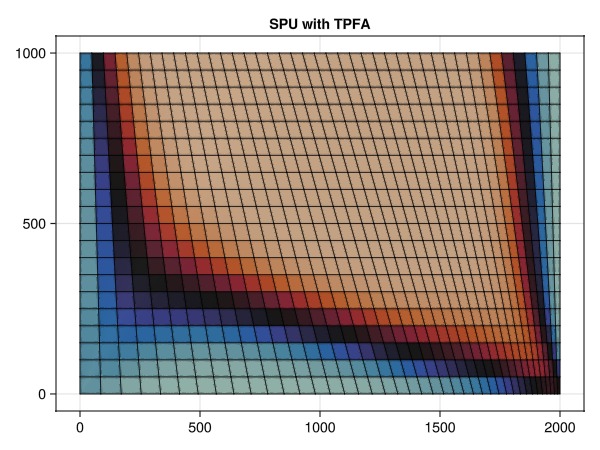

Simulate SPU-AvgMPFA

The next simulation uses a type of multi-point flux approximation (AverageMPFA or AvgMPFA), which is one class of consistent discretizations. As the scheme is consistent, the effect of the skewed grid is significantly reduced, with the remaining error being due to the coarse mesh chosen for illustrative purposes. Using AverageMPFA does not alleviate the smearing of the fluid front, however.

simulate_and_plot_discretizations(:spu, :avgmpfa)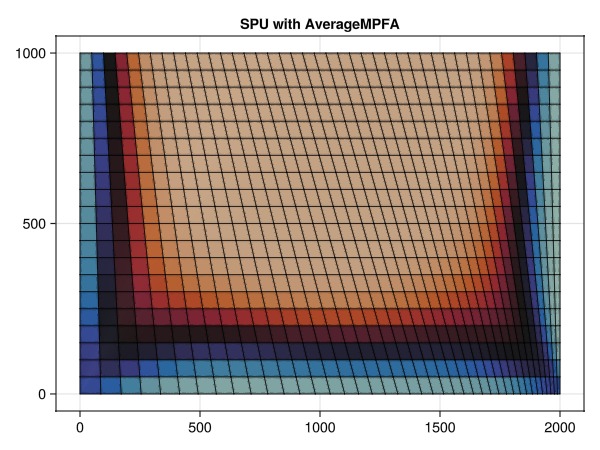

Simulate SPU-TPFA

The next simulation uses a nonlinear two-point flux approximation (NTPFA). This scheme is consistent and monotone, and can be derived from the AverageMPFA scheme by allowing the ratio between the two half-face fluxes at each interface to vary based on pressure.

simulate_and_plot_discretizations(:spu, :ntpfa)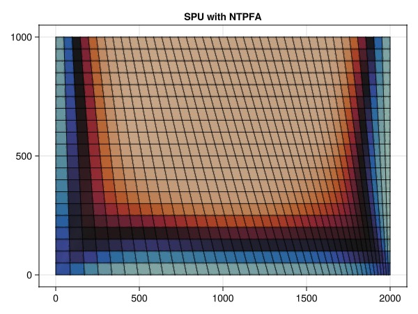

Simulate WENO-TPFA

The penultimate simulation uses a high-resolution scheme (WENO) for the flow, but reverts back to the inconsistent TPFA scheme for the pressure gradient. We now see significantly sharper fronts, but the bias towards the producer in the lower right corner is now back.

simulate_and_plot_discretizations(:weno, :tpfa)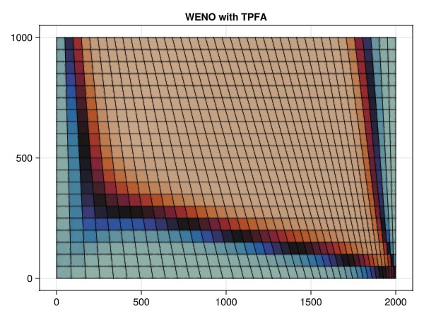

Simulate WENO-AvgMPFA

The final simulation combines the high-resolution WENO scheme with the consistent AverageMPFA scheme. The result is a sharp fluid front with no bias towards either producer. This is the most accurate simulation of the four for this intentionally badly gridded problem.

simulate_and_plot_discretizations(:weno, :avgmpfa)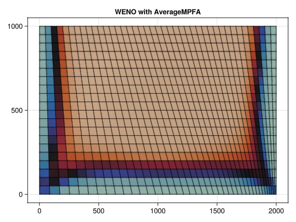

Compare the results

We can now compare the results of the different discretizations. We start by plotting the well curves in the two producers. Recall that the model is, from a flow perspective, completely symmetric, and the water cut in the two producers should be identical if the problem is fully resolved. We observe this for the consistent schemes, and delayed breakthrough for the SPU solves.

fig = Figure()
ax1 = Axis(fig[1, 1], title = "P1 water cut")
ax2 = Axis(fig[2, 1], title = "P2 water cut")
colors = Makie.wong_colors()
for (i, pr) in enumerate(all_results)
    name, result = pr
    ws, states = result
    wcut1 = ws[:P1][:wcut]
    wcut2 = ws[:P2][:wcut]
    lines!(ax1, wcut1, label = "$name", color = colors[i])
    lines!(ax2, wcut2, label = "$name", color = colors[i])
end
axislegend(ax1, position = :lt)
fig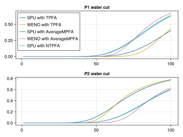

Compare the saturation fields as contours

We can also compare the saturation fields for the different discretizations to see the spatial differences. To make life a bit easier, we make a function to do the comparison plots for us.

function compare_contours(name1, name2, title)
    cmp = :seaborn_icefire_gradient
    r1 = all_results[name1]
    r2 = all_results[name2]
    fig = Figure(size = (1200, 800))
    ax = Axis(fig[1, 1], title = title)
    s1 = reshape(r1.states[75][:Saturations][1, :], nx, ny)
    s2 = reshape(r2.states[75][:Saturations][1, :], nx, ny)

    contourf!(ax, s2, colormap = cmp, label = name2)
    contour!(ax, s1, color = :white, linewidth = 5)
    contour!(ax, s1, colormap = cmp, linewidth = 3, label = name1)
    axislegend(position = :ct)

    axd = Axis(fig[1, 2], title = "Difference")
    plt = contourf!(axd, s1-s2,
        colormap = :seismic,
        label = name2,
        levels = range(-1, 1, length = 10),
        colorscale = (-1.0, 1.0)
    )
    Colorbar(fig[1, 3], limits = (-1, 1), colormap = :seismic)
    Colorbar(fig[2, 1:3], limits = (-1, 1), colormap = cmp, vertical = false)

    ax1 = Axis(fig[3, 1], title = name1)
    contourf!(ax1, s1, colormap = cmp)

    ax2 = Axis(fig[3, 2], title = name2)
    contourf!(ax2, s2, colormap = cmp)
    fig
end

compare_contours (generic function with 1 method)

Compare SPU-TPFA and SPU-AvgMPFA

compare_contours("SPU with AverageMPFA", "SPU with TPFA", "Consistent (AvgMPFA) vs inconsistent (TPFA)")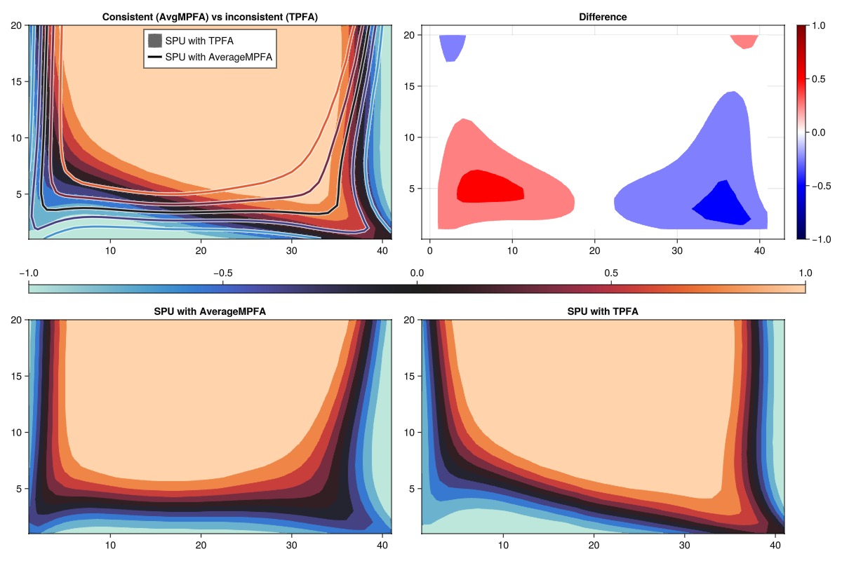

Compare WENO-TPFA and SPU-TPFA

compare_contours("WENO with TPFA", "SPU with TPFA", "High resolution (WENO) vs first order (SPU)")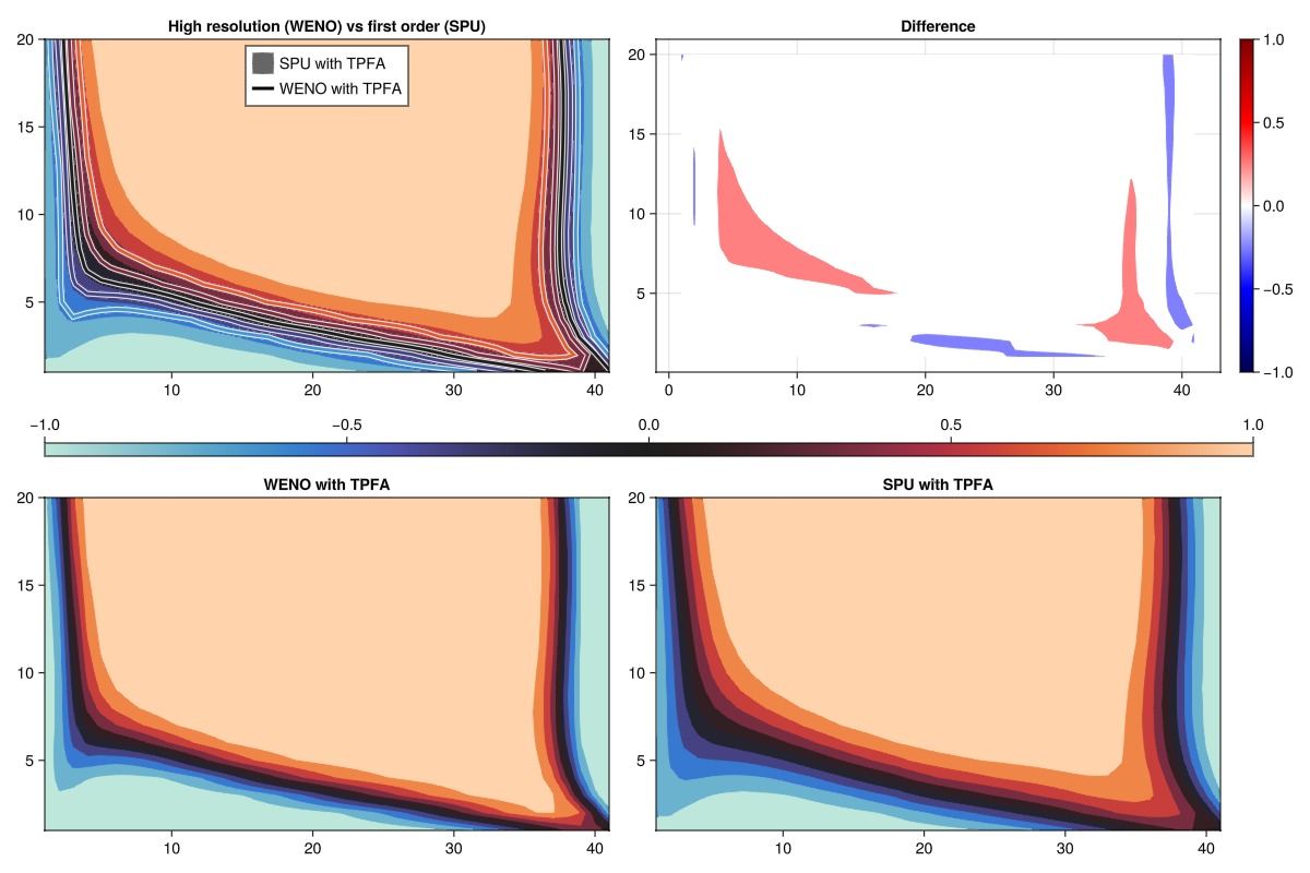

Compare WENO-AvgMPFA and SPU-TPFA

compare_contours("WENO with AverageMPFA", "SPU with TPFA", "High resolution + consistent vs first order + inconsistent")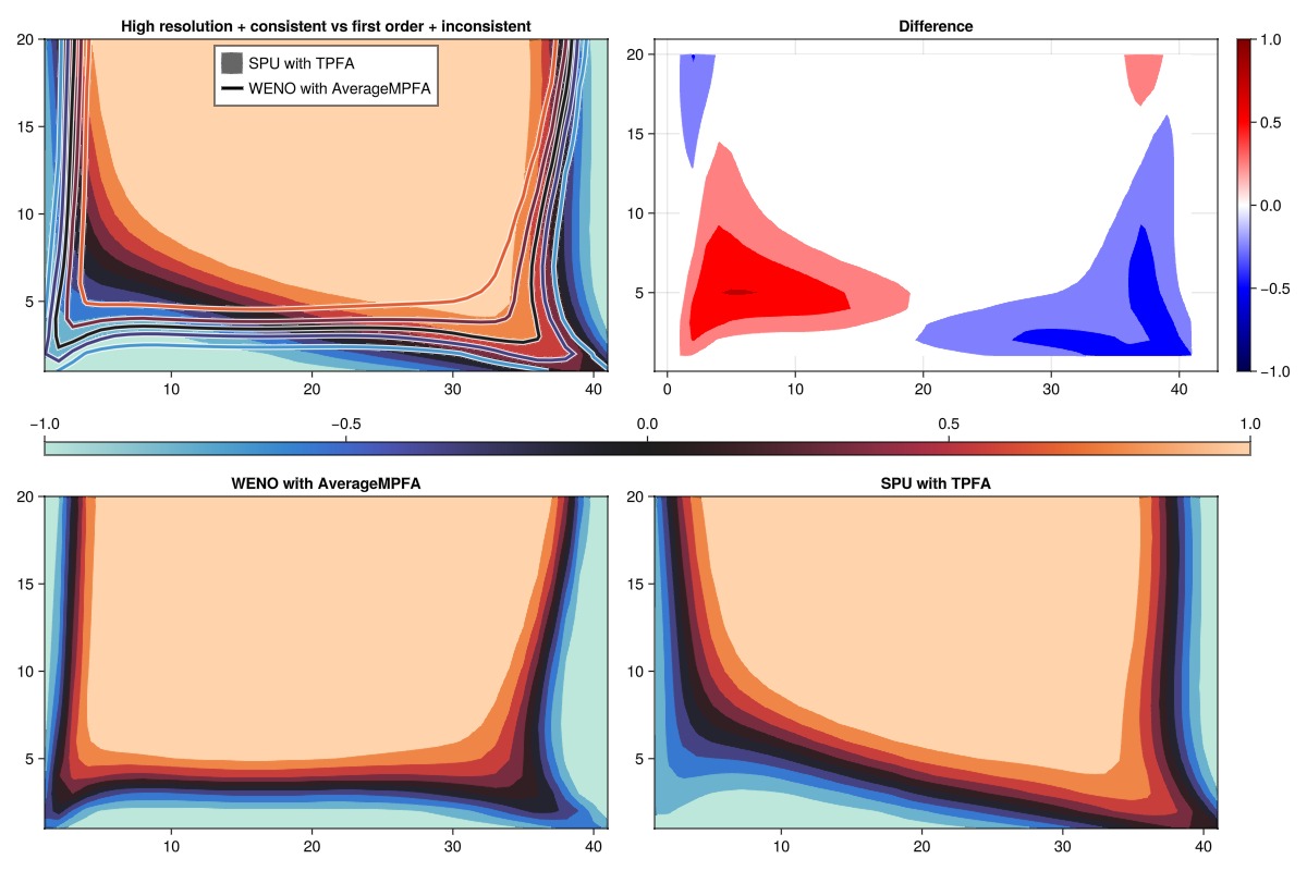

Conclusion

The example demonstrates how different discretizations can affect the results of a simulation. The example is intentionally set up to show the differences in the discretizations. The results show that the consistent discretizations (AvgMPFA and NTPFA) can reduce the bias from grid orientation, and, while not present here, permeability tensor effects. The high-resolution WENO scheme can be employed to reduce smearing of the fluid fronts, which is important for problems that are not self-sharpening (e.g. compositional flow and miscible displacements).

These schemes are not a pancea, however, as they require more computational effort to linearize and can have robustness issues where nonlinear convergence rates deteriorate and shorter timesteps may be required. They are accessible in JutulDarcy through the high-level interface and can be applied to any mesh and physics combination supported by the rest of the solvers.

We plot a summary of the saturation fields for all combinations of a pair of consistent and a pair of inconsistent discretizations to demonstrate the key differences.

fig = Figure(size = (1200, 800))
function plot_sat!(i, j, name)
    sg = all_results[name].states[75][:Saturations][1, :]
    ax = Axis(fig[i,j])
    hidespines!(ax)
    hidedecorations!(ax)
    plt = plot_cell_data!(ax, g, sg, colormap = :seaborn_icefire_gradient, colorrange = (0.0, 1.0))
    Jutul.plot_mesh_edges!(ax, g)
    return plt
end
Label(fig[0, 1], "Single-point upwind", fontsize = 30, tellheight = true, tellwidth = false)
Label(fig[0, 2], "High resolution", fontsize = 30, tellheight = true, tellwidth = false)

Label(fig[1, 0], "TPFA", fontsize = 30, rotation = pi/2, tellheight = false, tellwidth = true)
Label(fig[2, 0], "AverageMPFA", fontsize = 30, rotation = pi/2, tellheight = false, tellwidth = true)

plot_sat!(1, 1, "SPU with TPFA")
plot_sat!(2, 1, "SPU with AverageMPFA")
plot_sat!(1, 2, "WENO with TPFA")
plt = plot_sat!(2, 2, "WENO with AverageMPFA")
Colorbar(fig[:, 3], plt)
fig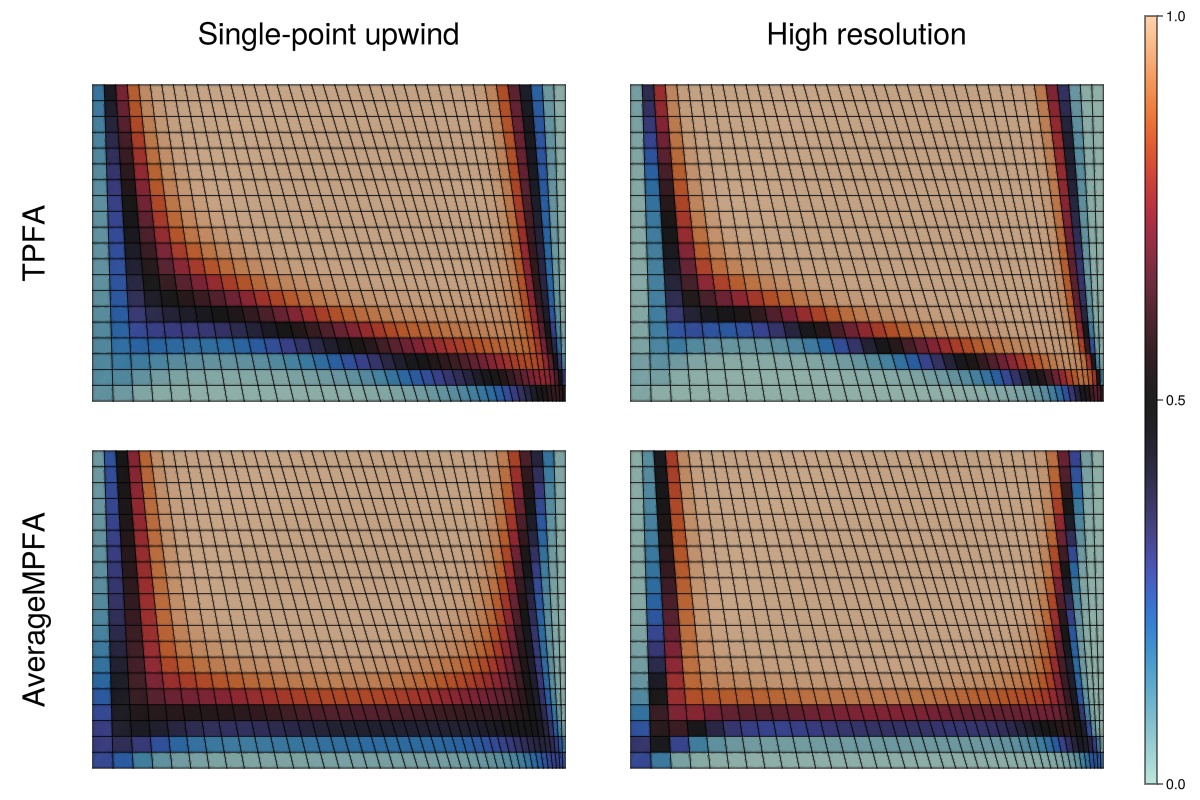

Example on GitHub

If you would like to run this example yourself, it can be downloaded from the JutulDarcy.jl GitHub repository as a script, or as a Jupyter Notebook

This example took 61.862253822 seconds to complete.

---

This page was generated using Literate.jl.