Polymer injection in a 2D black-oil reservoir model
Blackoil Tracers Validation InputFileThis example validates a small polymer model taken from the OPM-tests repository. The model is a 2D black-oil reservoir model with polymer injection. Adding polymer to the water phase increases the viscosity of the water and helps with mobility control. This is implemented in JutulDarcy as a tracer that can alter the properties of the system.
At present, the JutulDarcy polymer model supports the following features:
Polymer injection in the water phase
Varying degree of mixing between polymer and water
Adsorption of polymer to the rock
Polymer viscosity changes
Permeability reduction from polymer
Dead pore space for polymer part of water phase
Note that non-Newtonian rheology / shear effects are not yet implemented in the polymer model.
using GeoEnergyIO, Jutul, JutulDarcy, GLMakie, DelimitedFiles
pth = JutulDarcy.GeoEnergyIO.test_input_file_path("BOPOLYMER_NOSHEAR", "BOPOLYMER_NOSHEAR.DATA")
data = parse_data_file(pth)
case = setup_case_from_data_file(data)
push!(case.model[:Reservoir].output_variables, :PolymerConcentration)
push!(case.model[:Reservoir].output_variables, :PhaseViscosities)
push!(case.model[:Reservoir].output_variables, :AdsorbedPolymerConcentration)

ws, states, time = simulate_reservoir(case)
ReservoirSimResult with 228 entries:
wells (2 present):
:PROD01
:INJE01
Results per well:
:wrat => Vector{Float64} of size (228,)
:Aqueous_mass_rate => Vector{Float64} of size (228,)
:orat => Vector{Float64} of size (228,)
:bhp => Vector{Float64} of size (228,)
:mrat => Vector{Float64} of size (228,)
:gor => Vector{Float64} of size (228,)
:lrat => Vector{Float64} of size (228,)
:mass_rate => Vector{Float64} of size (228,)
:rate => Vector{Float64} of size (228,)
:Vapor_mass_rate => Vector{Float64} of size (228,)
:control => Vector{Symbol} of size (228,)
:Liquid_mass_rate => Vector{Float64} of size (228,)
:wcut => Vector{Float64} of size (228,)
:grat => Vector{Float64} of size (228,)
states (Vector with 228 entries, reservoir variables for each state)
:Pressure => Vector{Float64} of size (100,)
:ImmiscibleSaturation => Vector{Float64} of size (100,)
:BlackOilUnknown => Vector{BlackOilX{Float64}} of size (100,)
:TotalMasses => Matrix{Float64} of size (3, 100)
:Rs => Vector{Float64} of size (100,)
:Rv => Vector{Float64} of size (100,)
:Saturations => Matrix{Float64} of size (3, 100)
:TracerMasses => Matrix{Float64} of size (1, 100)
:TracerConcentrations => Matrix{Float64} of size (1, 100)
:PolymerConcentration => Vector{Float64} of size (100,)
:PhaseViscosities => Matrix{Float64} of size (3, 100)
:AdsorbedPolymerConcentration => Vector{Float64} of size (100,)
time (report time for each state)
Vector{Float64} of length 228
result (extended states, reports)
SimResult with 228 entries
extra
Dict{Any, Any} with keys :simulator, :config
Completed at Jul. 10 2026 15:04 after 22 seconds, 539 milliseconds, 723.3 microseconds.Load the reference solution and set up plotting
ref_pth = JutulDarcy.GeoEnergyIO.test_input_file_path("BOPOLYMER_NOSHEAR", "result.txt")
tab, header = DelimitedFiles.readdlm(ref_pth, header = true)
header = vec(header)
units = tab[1, :]
tab = Float64.(tab[2:end, :])
getcol(x) = tab[:, findfirst(isequal(x), header)]
time_ref = getcol("TIME")

function plot_comparison(jutul, ref, label; pos = :rt)
    fig = Figure()
    ax = Axis(fig[1, 1]; xlabel = "Time / days", ylabel = label)
    lines!(ax, time_ref, ref, label = "Reference", color = :black)
    lines!(ax, time./si_unit(:day), jutul, label = "JutulDarcy", linestyle = :dash, linewidth = 2, color = :black)
    lines!(ax, [1285.0, 1285.0], [minimum([jutul; ref]), maximum([jutul; ref])], label = "Polymer injection start", color = :red)
    lines!(ax, [2960.0, 2960.0], [minimum([jutul; ref]), maximum([jutul; ref])], label = "Polymer injection stops", color = :blue)
    axislegend(position = pos)
    fig
end
plot_comparison (generic function with 1 method)Plot oil production rate
wopr_ref = getcol("WOPR:PROD01")
wopr = -ws[:PROD01, :orat]*si_unit(:day)
plot_comparison(wopr, wopr_ref, "Oil production rate / sm³/day")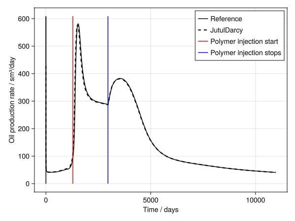
Plot bottom hole pressure
The pressure required to inject water significantly increases as polymer is added. This is due to the increased viscosity of the water phase when polymer is part of the mixture.
wbhp_ref = getcol("WBHP:INJE01")
wbhp = ws[:INJE01, :bhp]./si_unit(:bar)
plot_comparison(wbhp, wbhp_ref, "Injector bottom hole pressure / bar", pos = :rb)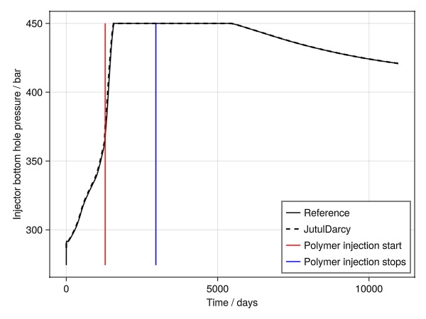
Plot the water front after polymer injection
reservoir = reservoir_domain(case.model)
g = physical_representation(reservoir)
UnstructuredMesh with 100 cells, 175 faces and 250 boundary facesPlot the water saturation front
fig, ax, plt = plot_cell_data(g, states[148][:Saturations][1, :])
ax.azimuth = 1.5π
ax.elevation = 0
hidedecorations!(ax)
fig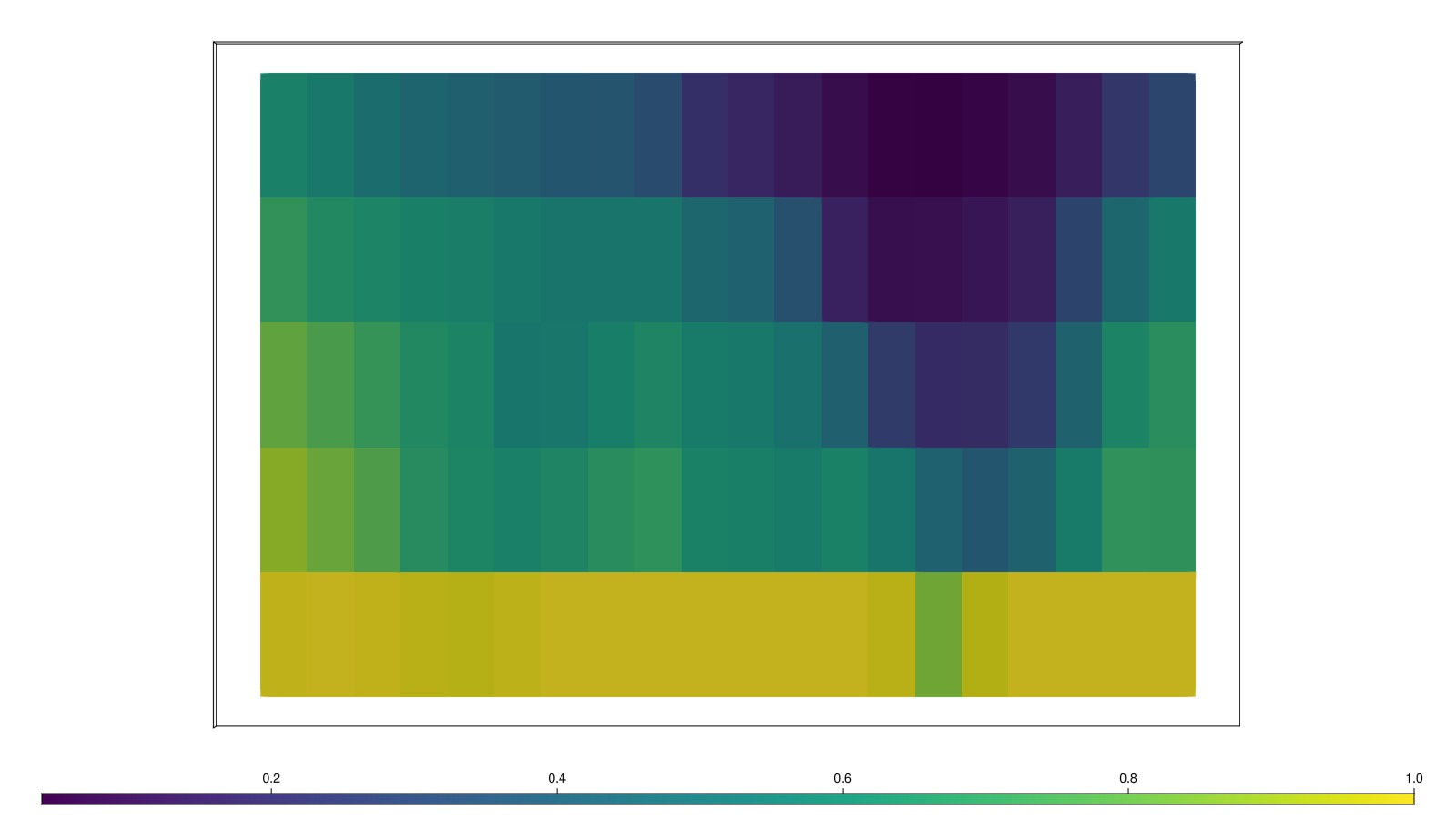
Plot the polymer concentration
fig, ax, plt = plot_cell_data(g, states[148][:PolymerConcentration])
ax.azimuth = 1.5π
ax.elevation = 0
hidedecorations!(ax)
fig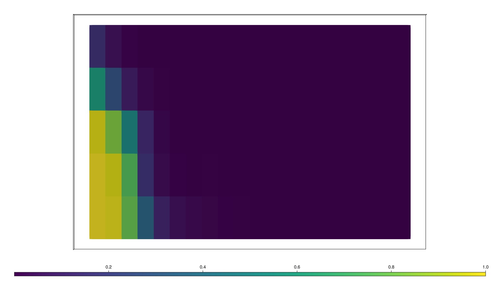
Plot the adsorbed polymer concentration
The polymer is adsorbed to the rock surface. This is a key part of the polymer model – the polymer is not only in the water phase but also adsorbed to the rock.
fig, ax, plt = plot_cell_data(g, states[148][:AdsorbedPolymerConcentration])
ax.azimuth = 1.5π
ax.elevation = 0
hidedecorations!(ax)
fig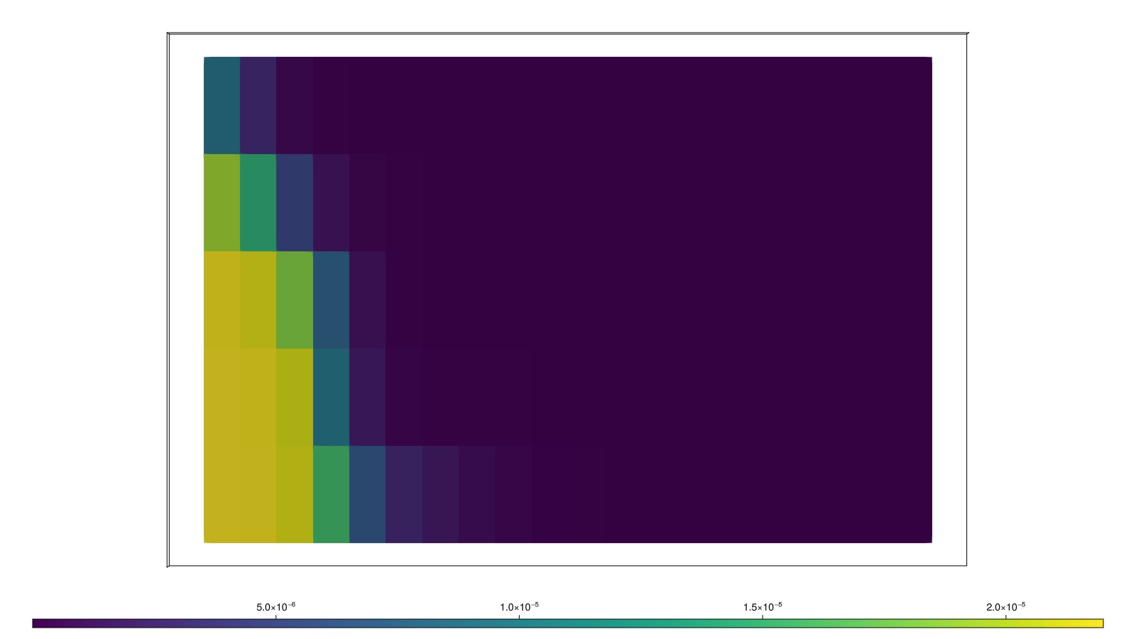
Example on GitHub
If you would like to run this example yourself, it can be downloaded from the JutulDarcy.jl GitHub repository as a script
This example took 75.511419618 seconds to complete.This page was generated using Literate.jl.