History matching a coarse model - CGNet
Immiscible HistoryMatchingThis example demonstrates how to calibrate a coarse model against results from a fine model. We do this by optimizing the parameters of the coarse model to match the well curves. This is a implementation of the method described in [7]. This also serves as a demonstration of how to use the simulator for history matching, as the fine model results can stand in for real field observations.
Load and simulate Egg base case
We take a subset of the first 60 steps (1350 days) since not much happens after that in terms of well behavior.
using Jutul, JutulDarcy, GeoEnergyIO, GLMakie
import LBFGSB as lb

egg_dir = JutulDarcy.GeoEnergyIO.test_input_file_path("EGG")
data_pth = joinpath(egg_dir, "EGG.DATA")

fine_case = setup_case_from_data_file(data_pth)
fine_case = fine_case[1:60]
simulated_fine = simulate_reservoir(fine_case)
plot_reservoir(fine_case, simulated_fine.states, key = :Saturations, step = 60)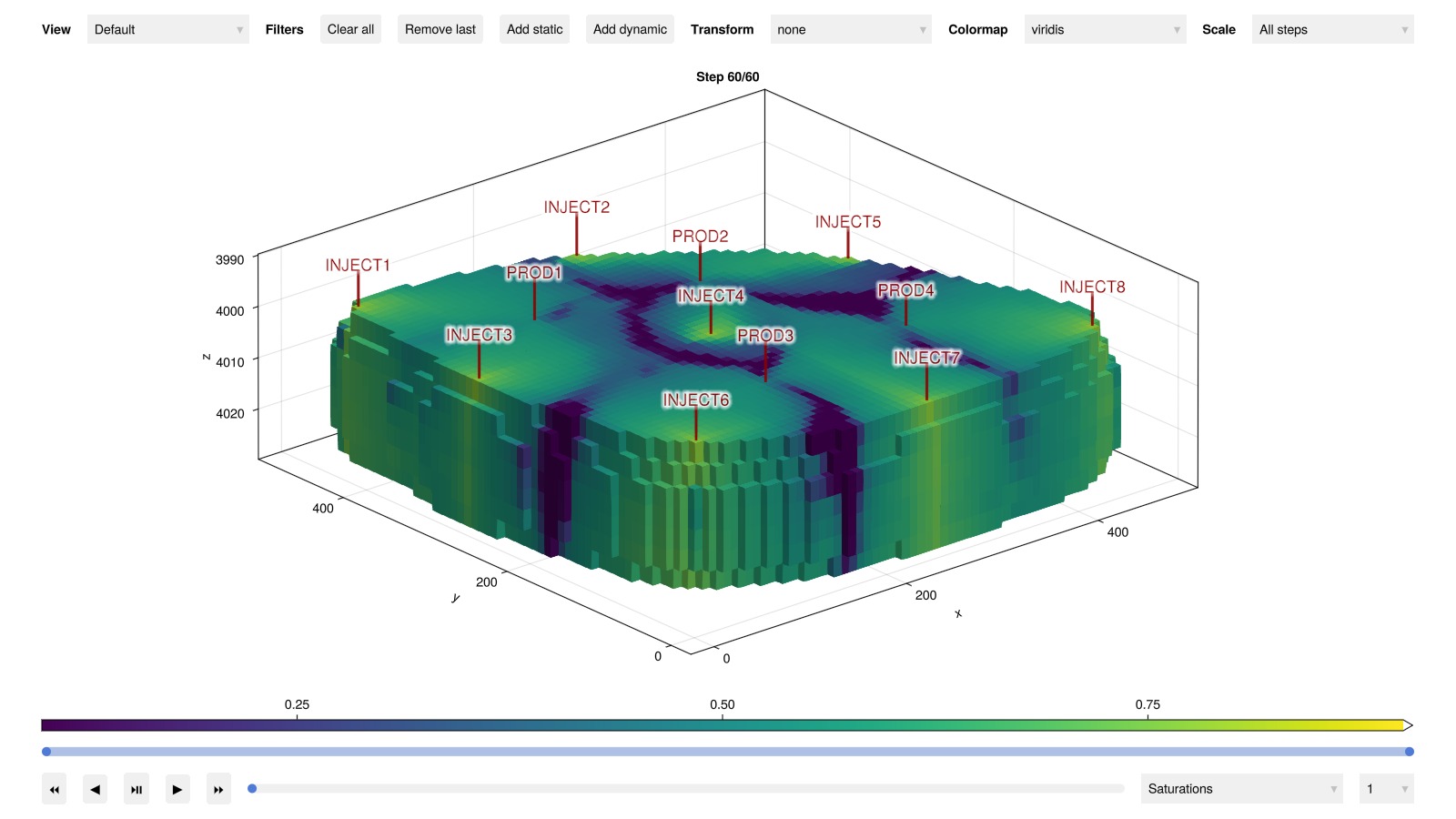
Create initial coarse model and simulate
coarse_case = JutulDarcy.coarsen_reservoir_case(fine_case, (25, 25, 5), method = :ijk)
simulated_coarse = simulate_reservoir(coarse_case)
plot_reservoir(coarse_case, simulated_coarse.states, key = :Saturations, step = 60)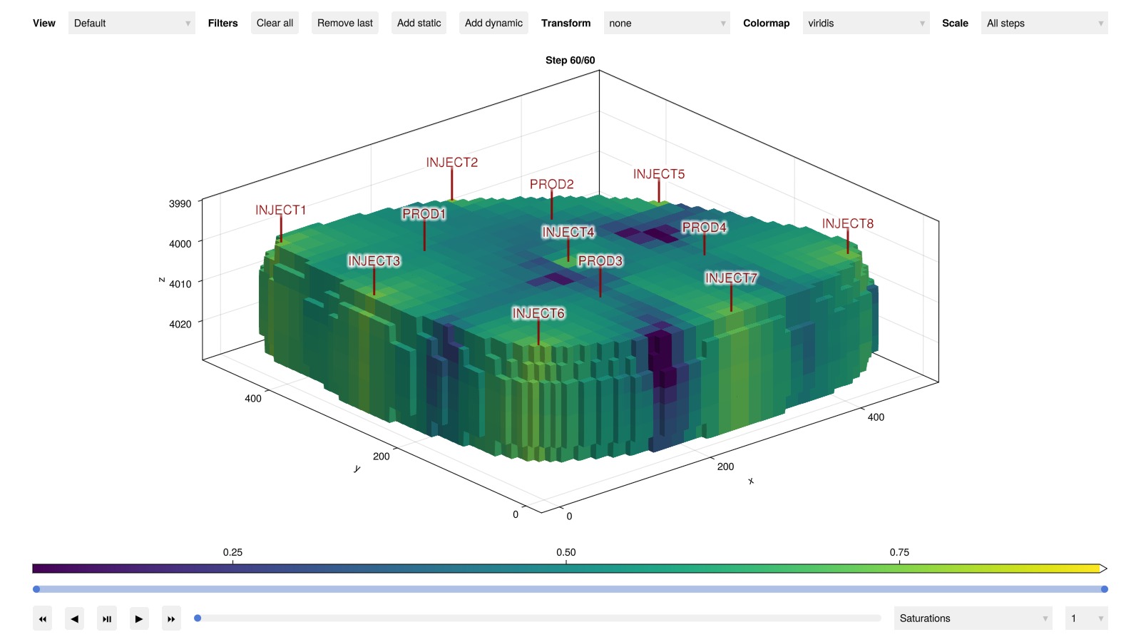
Setup optimization
We set up the optimization problem by defining the objective function as a sum of squared mismatches for all well observations, for all time-steps. We also define limits for the parameters, and set up the optimization problem.
We also limit the number of function evaluations since this example runs as a part of continuous integration and we want to keep the runtime short.
function setup_optimization_cgnet(case_c, case_f, result_f)
    states_f = result_f.result.states
    wells_results, = result_f
    model_c = case_c.model
    state0_c = setup_state(model_c, case_c.state0);
    param_c = setup_parameters(model_c)
    forces_c = case_c.forces
    dt = case_c.dt
    model_f = case_f.model

    bhp = JutulDarcy.BottomHolePressureTarget(1.0)
    wells = collect(keys(JutulDarcy.get_model_wells(case_f)))

    day = si_unit(:day)
    wrat_scale = (1/150)*day
    orat_scale = (1/80)*day
    grat_scale = (1/1000)*day

    w = []
    matches = []
    signs = []
    sys = reservoir_model(model_f).system
    wrat = SurfaceWaterRateTarget(-1.0)
    orat = SurfaceOilRateTarget(-1.0)
    grat = SurfaceGasRateTarget(-1.0)

    push!(matches, bhp)
    push!(w, 1.0/si_unit(:bar))
    push!(signs, 1)

    for phase in JutulDarcy.get_phases(sys)
        if phase == LiquidPhase()
            push!(matches, orat)
            push!(w, orat_scale)
            push!(signs, -1)

        elseif phase == VaporPhase()
            push!(matches, grat)
            push!(w, grat_scale)
            push!(signs, -1)
        else
            @assert phase == AqueousPhase()
            push!(matches, wrat)
            push!(w, wrat_scale)
            push!(signs, -1)
        end
    end
    signs = zeros(Int, length(signs))
    o_scale = 1.0/(sum(dt)*length(wells))
    G = (model_c, state_c, dt, step_info, forces) -> well_mismatch(
        matches,
        wells,
        model_f,
        states_f,
        model_c,
        state_c,
        dt,
        step_info,
        forces,
        weights = w,
        scale = o_scale,
        signs = signs
    )

    @assert Jutul.evaluate_objective(G, model_f, states_f, dt, case_f.forces) == 0.0
    #
    cfg = optimization_config(model_c, param_c,
        use_scaling = true,
        rel_min = 0.001,
        rel_max = 1000
    )
    for (k, v) in cfg
        for (ki, vi) in v
            if ki == :FluidVolume
                vi[:active] = k == :Reservoir
            end
            if ki == :ConnateWater
                vi[:active] = false
            end
            if ki in [:TwoPointGravityDifference, :PhaseViscosities, :PerforationGravityDifference]
                vi[:active] = false
            end
            if ki in [:WellIndices, :Transmissibilities]
                vi[:active] = true
                vi[:abs_min] = 0.0
                vi[:abs_max] = 1e-6
            end

        end
    end
    opt_setup = setup_parameter_optimization(model_c, state0_c, param_c, dt, forces_c, G, cfg);
    x0 = opt_setup.x0
    F0 = opt_setup.F!(x0)
    dF0 = opt_setup.dF!(similar(x0), x0)
    println("Initial objective: $F0, gradient norm $(sum(abs, dF0))")
    return opt_setup
end
setup_optimization_cgnet (generic function with 1 method)Define the optimization loop
JutulDarcy can use any optimization package that can work with gradients and limits, here we use the LBFGSB package.
function optimize_cgnet(opt_setup)
    lower = opt_setup.limits.min
    upper = opt_setup.limits.max
    x0 = opt_setup.x0
    n = length(x0)
    setup = Dict(:lower => lower, :upper => upper, :x0 => copy(x0))

    prt = 1
    f! = (x) -> opt_setup.F_and_dF!(NaN, nothing, x)
    g! = (dFdx, x) -> opt_setup.F_and_dF!(NaN, dFdx, x)
    results, final_x = lb.lbfgsb(f!, g!, x0, lb=lower, ub=upper,
        iprint = prt,
        factr = 1e12,
        maxfun = 20,
        maxiter = 20,
        m = 20
    )
    return (final_x, results, setup)
end
optimize_cgnet (generic function with 1 method)Run the optimization
opt_setup = setup_optimization_cgnet(coarse_case, fine_case, simulated_fine);
final_x, results, setup = optimize_cgnet(opt_setup);
Parameters for PROD4
┌─────────────┬──────────────┬───┬─────────┬─────────────┬────────────────┬─────
│ Name │ Entity │ N │ Scale │ Abs. limits │ Rel. limits │ ⋯
├─────────────┼──────────────┼───┼─────────┼─────────────┼────────────────┼─────
│ WellIndices │ Perforations │ 5 │ default │ [0, 1e-06] │ [0.001, 1e+03] │ [4 ⋯
└─────────────┴──────────────┴───┴─────────┴─────────────┴────────────────┴─────
3 columns omitted
Parameters for Reservoir
┌────────────────────┬────────┬──────┬─────────┬─────────────────┬──────────────
│ Name │ Entity │ N │ Scale │ Abs. limits │ Rel. lim ⋯
├────────────────────┼────────┼──────┼─────────┼─────────────────┼──────────────
│ Transmissibilities │ Faces │ 6792 │ default │ [0, 1e-06] │ [0.001, 1e+ ⋯
│ FluidVolume │ Cells │ 2516 │ default │ [2.22e-16, Inf] │ [0.001, 1e+ ⋯
└────────────────────┴────────┴──────┴─────────┴─────────────────┴──────────────
4 columns omitted
Parameters for INJECT5
┌─────────────┬──────────────┬───┬─────────┬─────────────┬────────────────┬─────
│ Name │ Entity │ N │ Scale │ Abs. limits │ Rel. limits │ ⋯
├─────────────┼──────────────┼───┼─────────┼─────────────┼────────────────┼─────
│ WellIndices │ Perforations │ 5 │ default │ [0, 1e-06] │ [0.001, 1e+03] │ [9 ⋯
└─────────────┴──────────────┴───┴─────────┴─────────────┴────────────────┴─────
3 columns omitted
Parameters for INJECT4
┌─────────────┬──────────────┬───┬─────────┬─────────────┬────────────────┬─────
│ Name │ Entity │ N │ Scale │ Abs. limits │ Rel. limits │ ⋯
├─────────────┼──────────────┼───┼─────────┼─────────────┼────────────────┼─────
│ WellIndices │ Perforations │ 5 │ default │ [0, 1e-06] │ [0.001, 1e+03] │ [2 ⋯
└─────────────┴──────────────┴───┴─────────┴─────────────┴────────────────┴─────
3 columns omitted
Parameters for INJECT8
┌─────────────┬──────────────┬───┬─────────┬─────────────┬────────────────┬─────
│ Name │ Entity │ N │ Scale │ Abs. limits │ Rel. limits │ ⋯
├─────────────┼──────────────┼───┼─────────┼─────────────┼────────────────┼─────
│ WellIndices │ Perforations │ 5 │ default │ [0, 1e-06] │ [0.001, 1e+03] │ [2 ⋯
└─────────────┴──────────────┴───┴─────────┴─────────────┴────────────────┴─────
3 columns omitted
Parameters for INJECT6
┌─────────────┬──────────────┬───┬─────────┬─────────────┬────────────────┬─────
│ Name │ Entity │ N │ Scale │ Abs. limits │ Rel. limits │ ⋯
├─────────────┼──────────────┼───┼─────────┼─────────────┼────────────────┼─────
│ WellIndices │ Perforations │ 5 │ default │ [0, 1e-06] │ [0.001, 1e+03] │ [5 ⋯
└─────────────┴──────────────┴───┴─────────┴─────────────┴────────────────┴─────
3 columns omitted
Parameters for INJECT1
┌─────────────┬──────────────┬───┬─────────┬─────────────┬────────────────┬─────
│ Name │ Entity │ N │ Scale │ Abs. limits │ Rel. limits │ ⋯
├─────────────┼──────────────┼───┼─────────┼─────────────┼────────────────┼─────
│ WellIndices │ Perforations │ 5 │ default │ [0, 1e-06] │ [0.001, 1e+03] │ [4 ⋯
└─────────────┴──────────────┴───┴─────────┴─────────────┴────────────────┴─────
3 columns omitted
Parameters for INJECT7
┌─────────────┬──────────────┬───┬─────────┬─────────────┬────────────────┬─────
│ Name │ Entity │ N │ Scale │ Abs. limits │ Rel. limits │ ⋯
├─────────────┼──────────────┼───┼─────────┼─────────────┼────────────────┼─────
│ WellIndices │ Perforations │ 5 │ default │ [0, 1e-06] │ [0.001, 1e+03] │ [2 ⋯
└─────────────┴──────────────┴───┴─────────┴─────────────┴────────────────┴─────
3 columns omitted
Parameters for INJECT3
┌─────────────┬──────────────┬───┬─────────┬─────────────┬────────────────┬─────
│ Name │ Entity │ N │ Scale │ Abs. limits │ Rel. limits │ ⋯
├─────────────┼──────────────┼───┼─────────┼─────────────┼────────────────┼─────
│ WellIndices │ Perforations │ 5 │ default │ [0, 1e-06] │ [0.001, 1e+03] │ [4 ⋯
└─────────────┴──────────────┴───┴─────────┴─────────────┴────────────────┴─────
3 columns omitted
Parameters for PROD2
┌─────────────┬──────────────┬───┬─────────┬─────────────┬────────────────┬─────
│ Name │ Entity │ N │ Scale │ Abs. limits │ Rel. limits │ ⋯
├─────────────┼──────────────┼───┼─────────┼─────────────┼────────────────┼─────
│ WellIndices │ Perforations │ 5 │ default │ [0, 1e-06] │ [0.001, 1e+03] │ [2 ⋯
└─────────────┴──────────────┴───┴─────────┴─────────────┴────────────────┴─────
3 columns omitted
Parameters for PROD3
┌─────────────┬──────────────┬───┬─────────┬─────────────┬────────────────┬─────
│ Name │ Entity │ N │ Scale │ Abs. limits │ Rel. limits │ ⋯
├─────────────┼──────────────┼───┼─────────┼─────────────┼────────────────┼─────
│ WellIndices │ Perforations │ 5 │ default │ [0, 1e-06] │ [0.001, 1e+03] │ [2 ⋯
└─────────────┴──────────────┴───┴─────────┴─────────────┴────────────────┴─────
3 columns omitted
Parameters for PROD1
┌─────────────┬──────────────┬───┬─────────┬─────────────┬────────────────┬─────
│ Name │ Entity │ N │ Scale │ Abs. limits │ Rel. limits │ ⋯
├─────────────┼──────────────┼───┼─────────┼─────────────┼────────────────┼─────
│ WellIndices │ Perforations │ 5 │ default │ [0, 1e-06] │ [0.001, 1e+03] │ [2 ⋯
└─────────────┴──────────────┴───┴─────────┴─────────────┴────────────────┴─────
3 columns omitted
Parameters for INJECT2
┌─────────────┬──────────────┬───┬─────────┬─────────────┬────────────────┬─────
│ Name │ Entity │ N │ Scale │ Abs. limits │ Rel. limits │ ⋯
├─────────────┼──────────────┼───┼─────────┼─────────────┼────────────────┼─────
│ WellIndices │ Perforations │ 5 │ default │ [0, 1e-06] │ [0.001, 1e+03] │ [1 ⋯
└─────────────┴──────────────┴───┴─────────┴─────────────┴────────────────┴─────
3 columns omitted
Obj. #1: 5.9823e+00 (best: Inf, relative: 1.0000e+00)
Initial objective: 5.982337521402408, gradient norm 585603.2206290782
RUNNING THE L-BFGS-B CODE
* * *
Machine precision = 2.220D-16
N = 9368 M = 20
At X0 0 variables are exactly at the bounds
At iterate 0 f= 5.98234D+00 |proj g|= 9.99001D-01
┌ Warning: Partial data passed, objective set to large value 59.823375214024075.
└ @ Jutul ~/.julia/packages/Jutul/iu9It/src/simulator/optimization.jl:242
Obj. #2: 5.9823e+01 (best: 5.9823e+00, relative: 1.0000e+01)
┌ Warning: Mismatch in states and timesteps for adjoints.
└ @ Jutul ~/.julia/packages/Jutul/iu9It/src/simulator/optimization.jl:189
Obj. #3: 8.9778e+01 (best: 5.9823e+00, relative: 1.5007e+01)
Obj. #4: 8.8870e+01 (best: 5.9823e+00, relative: 1.4855e+01)
Obj. #5: 8.7062e+01 (best: 5.9823e+00, relative: 1.4553e+01)
Obj. #6: 8.1792e+01 (best: 5.9823e+00, relative: 1.3672e+01)
Obj. #7: 6.4626e+01 (best: 5.9823e+00, relative: 1.0803e+01)
Obj. #8: 2.7817e+01 (best: 5.9823e+00, relative: 4.6498e+00)
Obj. #9: 2.5897e+00 (best: 5.9823e+00, relative: 4.3290e-01)
At iterate 1 f= 2.58973D+00 |proj g|= 9.99000D-01
Obj. #10: 1.0977e+00 (best: 2.5897e+00, relative: 1.8349e-01)
At iterate 2 f= 1.09770D+00 |proj g|= 9.99002D-01
Obj. #11: 1.6713e+00 (best: 1.0977e+00, relative: 2.7938e-01)
Obj. #12: 3.2835e-01 (best: 1.0977e+00, relative: 5.4887e-02)
At iterate 3 f= 3.28354D-01 |proj g|= 9.99000D-01
Obj. #13: 2.6822e-01 (best: 3.2835e-01, relative: 4.4835e-02)
At iterate 4 f= 2.68218D-01 |proj g|= 9.98818D-01
Obj. #14: 1.9528e-01 (best: 2.6822e-01, relative: 3.2642e-02)
At iterate 5 f= 1.95276D-01 |proj g|= 9.98818D-01
Obj. #15: 1.2688e-01 (best: 1.9528e-01, relative: 2.1209e-02)
At iterate 6 f= 1.26880D-01 |proj g|= 9.99004D-01
Obj. #16: 1.1554e-01 (best: 1.2688e-01, relative: 1.9313e-02)
At iterate 7 f= 1.15535D-01 |proj g|= 9.99005D-01
Obj. #17: 9.6782e-02 (best: 1.1554e-01, relative: 1.6178e-02)
At iterate 8 f= 9.67817D-02 |proj g|= 9.99003D-01
Obj. #18: 8.4167e-02 (best: 9.6782e-02, relative: 1.4069e-02)
At iterate 9 f= 8.41665D-02 |proj g|= 9.98787D-01
Obj. #19: 1.0004e-01 (best: 8.4167e-02, relative: 1.6723e-02)
Obj. #20: 7.7844e-02 (best: 8.4167e-02, relative: 1.3012e-02)
At iterate 10 f= 7.78439D-02 |proj g|= 9.99010D-01
* * *
Tit = total number of iterations
Tnf = total number of function evaluations
Tnint = total number of segments explored during Cauchy searches
Skip = number of BFGS updates skipped
Nact = number of active bounds at final generalized Cauchy point
Projg = norm of the final projected gradient
F = final function value
* * *
N Tit Tnf Tnint Skip Nact Projg F
9368 10 20 9253 0 6 9.990D-01 7.784D-02
F = 7.7843860525965120E-002
STOP: TOTAL NO. of f AND g EVALUATIONS EXCEEDS LIMIT
Cauchy time 2.869E-03 seconds.
Subspace minimization time 2.625E-03 seconds.
Line search time 7.027E+01 seconds.
Total User time 7.156E+01 seconds.Transfer the results back
The optimization is generic and works on a single long vector that represents all our active parameters. We can devectorize this vector back into the nested representation used by the model itself and simulate.
tuned_case = deepcopy(opt_setup.data[:case])
model_c = coarse_case.model
model_f = fine_case.model
param_c = tuned_case.parameters
data = opt_setup.data
devectorize_variables!(param_c, model_c, final_x, data[:mapper], config = data[:config])


simulated_tuned = simulate_reservoir(tuned_case);
Jutul: Simulating 3 years, 36.32 weeks as 60 report steps
╭────────────────┬──────────┬──────────────┬──────────╮
│ Iteration type │ Avg/step │ Avg/ministep │ Total │
│ │ 60 steps │ 69 ministeps │ (wasted) │
├────────────────┼──────────┼──────────────┼──────────┤
│ Newton │ 4.18333 │ 3.63768 │ 251 (0) │
│ Linearization │ 5.33333 │ 4.63768 │ 320 (0) │
│ Linear solver │ 16.7667 │ 14.5797 │ 1006 (0) │
│ Precond apply │ 33.5333 │ 29.1594 │ 2012 (0) │
╰────────────────┴──────────┴──────────────┴──────────╯
╭───────────────┬────────┬────────────┬────────╮
│ Timing type │ Each │ Relative │ Total │
│ │ ms │ Percentage │ s │
├───────────────┼────────┼────────────┼────────┤
│ Properties │ 0.3472 │ 3.97 % │ 0.0871 │
│ Equations │ 0.5323 │ 7.76 % │ 0.1703 │
│ Assembly │ 0.6047 │ 8.81 % │ 0.1935 │
│ Linear solve │ 0.4452 │ 5.09 % │ 0.1117 │
│ Linear setup │ 3.9714 │ 45.39 % │ 0.9968 │
│ Precond apply │ 0.2152 │ 19.72 % │ 0.4331 │
│ Update │ 0.1999 │ 2.28 % │ 0.0502 │
│ Convergence │ 0.3034 │ 4.42 % │ 0.0971 │
│ Input/Output │ 0.0691 │ 0.22 % │ 0.0048 │
│ Other │ 0.2059 │ 2.35 % │ 0.0517 │
├───────────────┼────────┼────────────┼────────┤
│ Total │ 8.7503 │ 100.00 % │ 2.1963 │
╰───────────────┴────────┴────────────┴────────╯Plot the results interactively
using GLMakie

wells_f, = simulated_fine
wells_c, = simulated_coarse
wells_t, states_t, time = simulated_tuned

plot_well_results([wells_f, wells_c, wells_t], time, names = ["Fine", "CGNet-initial", "CGNet-tuned"])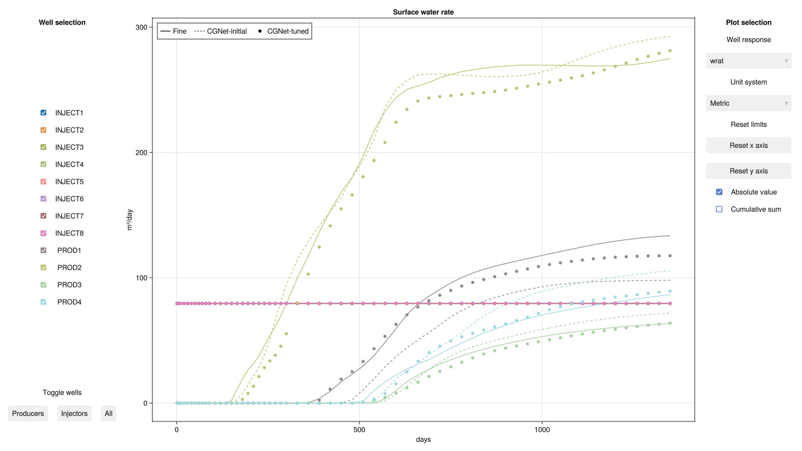
Create a function to compare individual wells
We next compare individual wells to see how the optimization has affected the match between the coarse scale and fine scale. As we can see, we have reasonably good match between the original model with about 18,000 cells and the coarse model with about 3000 cells. Even better match could be possible by adding more coarse blocks, or also optimizing for example the relative permeability parameters for the coarse model.
We plot the water cut and total rate for the production wells, and the bottom hole pressure for the injection wells.
function plot_tuned_well(k, kw; lposition = :lt)
    fig = Figure()
    ax = Axis(fig[1, 1], title = "$k", xlabel = "days", ylabel = "$kw")
    t = wells_f.time./si_unit(:day)
    if kw == :wcut
        F = x -> x[k, :wrat]./x[k, :lrat]
    else
        F = x -> abs.(x[k, kw])
    end

    lines!(ax, t, F(wells_f), label = "Fine-scale")
    lines!(ax, t, F(wells_c), label = "Initial coarse")
    lines!(ax, t, F(wells_t), label = "Tuned coarse")
    axislegend(position = lposition)
    fig
end
plot_tuned_well (generic function with 1 method)Plot PROD1 water cut
plot_tuned_well(:PROD1, :wcut)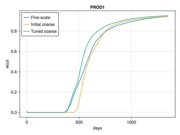
Plot PROD2 water cut
plot_tuned_well(:PROD2, :wcut)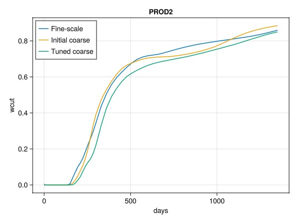
Plot PROD4 water cut
plot_tuned_well(:PROD4, :wcut)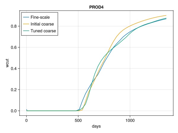
Plot PROD1 total rate
plot_tuned_well(:PROD1, :rate)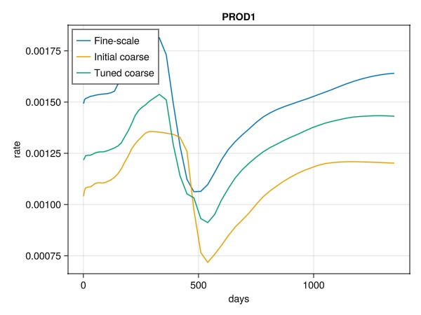
Plot PROD2 total rate
plot_tuned_well(:PROD2, :rate)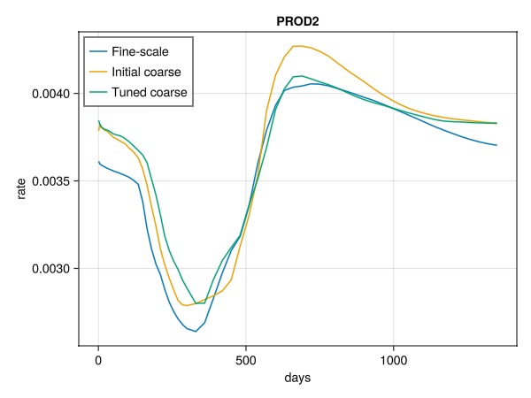
Plot PROD4 total rate
plot_tuned_well(:PROD4, :rate)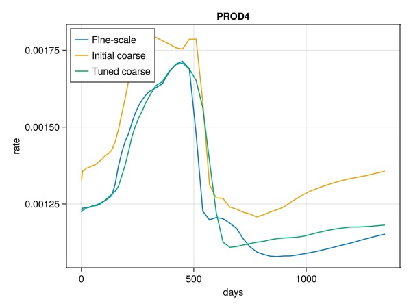
Plot INJECT1 bhp
plot_tuned_well(:INJECT1, :bhp, lposition = :rt)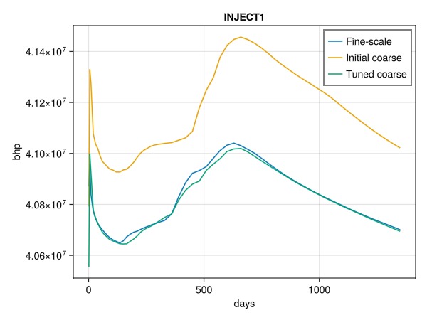
Plot INJECT4 bhp
plot_tuned_well(:INJECT4, :bhp, lposition = :rt)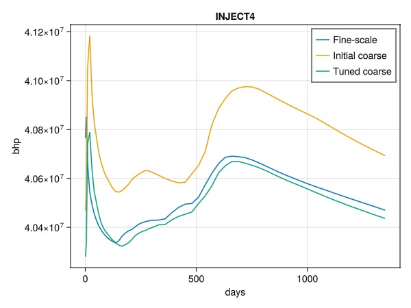
Plot the objective evaluations during optimization
fig = Figure()
ys = log10
is = x -> x
ax1 = Axis(fig[1, 1], yscale = ys, title = "Objective evaluations", xlabel = "Iterations", ylabel = "Objective")
plot!(ax1, opt_setup[:data][:obj_hist][2:end])
fig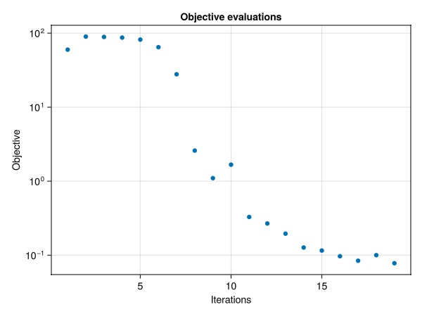
Plot the evoluation of scaled parameters
We show the difference between the initial and final values of the scaled parameters, as well as the lower bound.
JutulDarcy maps the parameters to a single vector for optimization with values that are approximately in the box limit range (0, 1). This is convenient for optimizers, but can also be useful when plotting the parameters, even if the units are not preserved in this visualization, only the magnitude.
fig = Figure(size = (800, 600))
ax1 = Axis(fig[1, 1], title = "Scaled parameters", ylabel = "Scaled value")
scatter!(ax1, setup[:x0], label = "Initial X")
scatter!(ax1, final_x, label = "Final X", markersize = 5)
lines!(ax1, setup[:lower], label = "Lower bound")
axislegend()

trans = data[:mapper][:Reservoir][:Transmissibilities]

function plot_bracket(v, k)
    start = v.offset_x+1
    stop = v.offset_x+v.n_x
    y0 = setup[:lower][start]
    y1 = setup[:lower][stop]
    bracket!(ax1, start, y0, stop, y1,
    text = "$k", offset = 1, orientation = :down)
end

for (k, v) in pairs(data[:mapper][:Reservoir])
    plot_bracket(v, k)
end
ylims!(ax1, (-0.2*maximum(final_x), nothing))
fig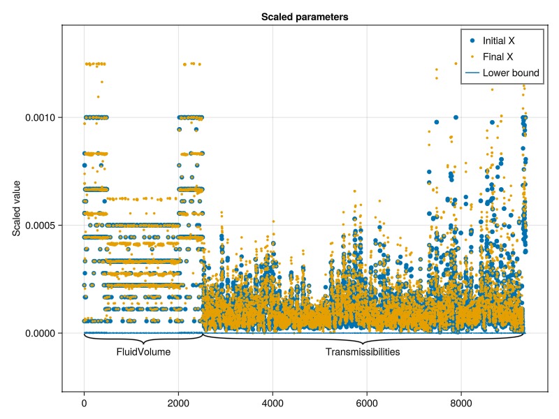
Example on GitHub
If you would like to run this example yourself, it can be downloaded from the JutulDarcy.jl GitHub repository as a script
This example took 209.821556001 seconds to complete.This page was generated using Literate.jl.