Aquifer thermal energy storage (ATES) validation
Geothermal Validation InputFileThis example validates JutulDarcy's thermal solver against results from a commercial simulator. The test case is a simple ATES model with a single pair of wells (hot / cold) where the cold well is used for pressure support with a mirrored injection rate. Towards the later part of the schedule, the cold well reinjects water that is a higher temperature than the background.
This case is completely specified in the ATES_TEST.DATA file which was provided by TNO. The model is a structured mesh with 472 500 active cells.
using Jutul, JutulDarcy, GeoEnergyIO, DelimitedFiles, GLMakie
basepth = GeoEnergyIO.test_input_file_path("ATES_TEST")
data = parse_data_file(joinpath(basepth, "ATES_TEST.DATA"))

wdata, wheader = readdlm(joinpath(basepth, "wells.txt"), ',', header = true)
cdata, cheader = readdlm(joinpath(basepth, "cells.txt"), ',', header = true)
case = setup_case_from_data_file(data)
ws, states, t_seconds = simulate_reservoir(case, info_level = 1);
Parser: PROPS/VISCREF - Parser has only partial support. VISCREF may have missing or wrong entries.
┌ Warning: Did not find supported time kw in step 126: Keys were ["WELOPEN"].
└ @ JutulDarcy ~/work/JutulDarcy.jl/JutulDarcy.jl/src/input_simulation/data_input.jl:1828
Jutul: Simulating 41 weeks, 5 days as 124 report steps
Step 1/124: Solving start to 2 days, Δt = 2 days
Step 2/124: Solving 2 days to 3 days, Δt = 1 day
Step 3/124: Solving 3 days to 4 days, Δt = 1 day
Step 4/124: Solving 4 days to 5 days, Δt = 1 day
Step 5/124: Solving 5 days to 6 days, Δt = 1 day
Step 6/124: Solving 6 days to 1 week, Δt = 1 day
Step 7/124: Solving 1 week to 1 week, 1 day, Δt = 1 day
Step 8/124: Solving 1 week, 1 day to 1 week, 2 days, Δt = 1 day
Step 9/124: Solving 1 week, 2 days to 1 week, 3 days, Δt = 1 day
Step 10/124: Solving 1 week, 3 days to 1 week, 4 days, Δt = 1 day
Step 11/124: Solving 1 week, 4 days to 1 week, 5 days, Δt = 1 day
Step 12/124: Solving 1 week, 5 days to 1 week, 6 days, Δt = 1 day
Step 13/124: Solving 1 week, 6 days to 2 weeks, Δt = 1 day
Step 14/124: Solving 2 weeks to 2 weeks, 1 day, Δt = 1 day
Step 15/124: Solving 2 weeks, 1 day to 2 weeks, 2 days, Δt = 1 day
Step 16/124: Solving 2 weeks, 2 days to 2 weeks, 3 days, Δt = 1 day
Step 17/124: Solving 2 weeks, 3 days to 2 weeks, 4 days, Δt = 1 day
Step 18/124: Solving 2 weeks, 4 days to 2 weeks, 5 days, Δt = 1 day
Step 19/124: Solving 2 weeks, 5 days to 2 weeks, 6 days, Δt = 1 day
Step 20/124: Solving 2 weeks, 6 days to 3 weeks, Δt = 1 day
Step 21/124: Solving 3 weeks to 3 weeks, 1 day, Δt = 1 day
Step 22/124: Solving 3 weeks, 1 day to 3 weeks, 2 days, Δt = 1 day
Step 23/124: Solving 3 weeks, 2 days to 3 weeks, 3 days, Δt = 1 day
Step 24/124: Solving 3 weeks, 3 days to 3 weeks, 4 days, Δt = 1 day
Step 25/124: Solving 3 weeks, 4 days to 3 weeks, 5 days, Δt = 1 day
Step 26/124: Solving 3 weeks, 5 days to 4 weeks, 3 days, Δt = 5 days
Step 27/124: Solving 4 weeks, 3 days to 4 weeks, 4 days, Δt = 1 day
Step 28/124: Solving 4 weeks, 4 days to 4 weeks, 5 days, Δt = 1 day
Step 29/124: Solving 4 weeks, 5 days to 5 weeks, 3 days, Δt = 5 days
Step 30/124: Solving 5 weeks, 3 days to 5 weeks, 4 days, Δt = 1 day
Step 31/124: Solving 5 weeks, 4 days to 5 weeks, 5 days, Δt = 1 day
Step 32/124: Solving 5 weeks, 5 days to 5 weeks, 6 days, Δt = 1 day
Step 33/124: Solving 5 weeks, 6 days to 6 weeks, 3 days, Δt = 4 days
Step 34/124: Solving 6 weeks, 3 days to 6 weeks, 4 days, Δt = 1 day
Step 35/124: Solving 6 weeks, 4 days to 6 weeks, 5 days, Δt = 1 day
Step 36/124: Solving 6 weeks, 5 days to 6 weeks, 6 days, Δt = 1 day
Step 37/124: Solving 6 weeks, 6 days to 7 weeks, Δt = 1 day
Step 38/124: Solving 7 weeks to 7 weeks, 1 day, Δt = 1 day
Step 39/124: Solving 7 weeks, 1 day to 7 weeks, 2 days, Δt = 1 day
Step 40/124: Solving 7 weeks, 2 days to 7 weeks, 3 days, Δt = 1 day
Step 41/124: Solving 7 weeks, 3 days to 7 weeks, 4 days, Δt = 1 day
Step 42/124: Solving 7 weeks, 4 days to 7 weeks, 5 days, Δt = 1 day
Step 43/124: Solving 7 weeks, 5 days to 7 weeks, 6 days, Δt = 1 day
Step 44/124: Solving 7 weeks, 6 days to 8 weeks, Δt = 1 day
Step 45/124: Solving 8 weeks to 8 weeks, 1 day, Δt = 1 day
Step 46/124: Solving 8 weeks, 1 day to 8 weeks, 2 days, Δt = 1 day
Step 47/124: Solving 8 weeks, 2 days to 8 weeks, 3 days, Δt = 1 day
Step 48/124: Solving 8 weeks, 3 days to 8 weeks, 4 days, Δt = 1 day
Step 49/124: Solving 8 weeks, 4 days to 8 weeks, 5 days, Δt = 1 day
Step 50/124: Solving 8 weeks, 5 days to 8 weeks, 6 days, Δt = 1 day
Step 51/124: Solving 8 weeks, 6 days to 9 weeks, Δt = 1 day
Step 52/124: Solving 9 weeks to 9 weeks, 1 day, Δt = 1 day
Step 53/124: Solving 9 weeks, 1 day to 9 weeks, 2 days, Δt = 1 day
Step 54/124: Solving 9 weeks, 2 days to 9 weeks, 3 days, Δt = 1 day
Step 55/124: Solving 9 weeks, 3 days to 9 weeks, 4 days, Δt = 1 day
Step 56/124: Solving 9 weeks, 4 days to 9 weeks, 5 days, Δt = 1 day
Step 57/124: Solving 9 weeks, 5 days to 9 weeks, 6 days, Δt = 1 day
Step 58/124: Solving 9 weeks, 6 days to 10 weeks, Δt = 1 day
Step 59/124: Solving 10 weeks to 10 weeks, 1 day, Δt = 1 day
Step 60/124: Solving 10 weeks, 1 day to 10 weeks, 2 days, Δt = 1 day
Step 61/124: Solving 10 weeks, 2 days to 10 weeks, 3 days, Δt = 1 day
Step 62/124: Solving 10 weeks, 3 days to 10 weeks, 4 days, Δt = 1 day
Step 63/124: Solving 10 weeks, 4 days to 10 weeks, 5 days, Δt = 1 day
Step 64/124: Solving 10 weeks, 5 days to 10 weeks, 6 days, Δt = 1 day
Step 65/124: Solving 10 weeks, 6 days to 11 weeks, Δt = 1 day
Step 66/124: Solving 11 weeks to 11 weeks, 1 day, Δt = 1 day
Step 67/124: Solving 11 weeks, 1 day to 11 weeks, 2 days, Δt = 1 day
Step 68/124: Solving 11 weeks, 2 days to 11 weeks, 3 days, Δt = 1 day
Step 69/124: Solving 11 weeks, 3 days to 11 weeks, 4 days, Δt = 1 day
Step 70/124: Solving 11 weeks, 4 days to 33 weeks, 2 days, Δt = 21 weeks, 5 days
Step 71/124: Solving 33 weeks, 2 days to 33 weeks, 3 days, Δt = 1 day
Step 72/124: Solving 33 weeks, 3 days to 33 weeks, 4 days, Δt = 1 day
Step 73/124: Solving 33 weeks, 4 days to 33 weeks, 5 days, Δt = 1 day
Step 74/124: Solving 33 weeks, 5 days to 33 weeks, 6 days, Δt = 1 day
Step 75/124: Solving 33 weeks, 6 days to 34 weeks, Δt = 1 day
Step 76/124: Solving 34 weeks to 34 weeks, 1 day, Δt = 1 day
Step 77/124: Solving 34 weeks, 1 day to 34 weeks, 2 days, Δt = 1 day
Step 78/124: Solving 34 weeks, 2 days to 34 weeks, 3 days, Δt = 1 day
Step 79/124: Solving 34 weeks, 3 days to 34 weeks, 4 days, Δt = 1 day
Step 80/124: Solving 34 weeks, 4 days to 34 weeks, 5 days, Δt = 1 day
Step 81/124: Solving 34 weeks, 5 days to 34 weeks, 6 days, Δt = 1 day
Step 82/124: Solving 34 weeks, 6 days to 35 weeks, Δt = 1 day
Step 83/124: Solving 35 weeks to 35 weeks, 1 day, Δt = 1 day
Step 84/124: Solving 35 weeks, 1 day to 35 weeks, 2 days, Δt = 1 day
Step 85/124: Solving 35 weeks, 2 days to 35 weeks, 3 days, Δt = 1 day
Step 86/124: Solving 35 weeks, 3 days to 35 weeks, 4 days, Δt = 1 day
Step 87/124: Solving 35 weeks, 4 days to 35 weeks, 5 days, Δt = 1 day
Step 88/124: Solving 35 weeks, 5 days to 35 weeks, 6 days, Δt = 1 day
Step 89/124: Solving 35 weeks, 6 days to 36 weeks, Δt = 1 day
Step 90/124: Solving 36 weeks to 36 weeks, 1 day, Δt = 1 day
Step 91/124: Solving 36 weeks, 1 day to 36 weeks, 2 days, Δt = 1 day
Step 92/124: Solving 36 weeks, 2 days to 36 weeks, 3 days, Δt = 1 day
Step 93/124: Solving 36 weeks, 3 days to 36 weeks, 4 days, Δt = 1 day
Step 94/124: Solving 36 weeks, 4 days to 36 weeks, 5 days, Δt = 1 day
Step 95/124: Solving 36 weeks, 5 days to 36 weeks, 6 days, Δt = 1 day
Step 96/124: Solving 36 weeks, 6 days to 37 weeks, Δt = 1 day
Step 97/124: Solving 37 weeks to 37 weeks, 1 day, Δt = 1 day
Step 98/124: Solving 37 weeks, 1 day to 37 weeks, 2 days, Δt = 1 day
Step 99/124: Solving 37 weeks, 2 days to 37 weeks, 3 days, Δt = 1 day
Step 100/124: Solving 37 weeks, 3 days to 37 weeks, 4 days, Δt = 1 day
Step 101/124: Solving 37 weeks, 4 days to 37 weeks, 5 days, Δt = 1 day
Step 102/124: Solving 37 weeks, 5 days to 37 weeks, 6 days, Δt = 1 day
Step 103/124: Solving 37 weeks, 6 days to 38 weeks, Δt = 1 day
Step 104/124: Solving 38 weeks to 38 weeks, 1 day, Δt = 1 day
Step 105/124: Solving 38 weeks, 1 day to 38 weeks, 2 days, Δt = 1 day
Step 106/124: Solving 38 weeks, 2 days to 38 weeks, 3 days, Δt = 1 day
Step 107/124: Solving 38 weeks, 3 days to 38 weeks, 4 days, Δt = 1 day
Step 108/124: Solving 38 weeks, 4 days to 38 weeks, 5 days, Δt = 1 day
Step 109/124: Solving 38 weeks, 5 days to 38 weeks, 6 days, Δt = 1 day
Step 110/124: Solving 38 weeks, 6 days to 39 weeks, Δt = 1 day
Step 111/124: Solving 39 weeks to 39 weeks, 1 day, Δt = 1 day
Step 112/124: Solving 39 weeks, 1 day to 39 weeks, 2 days, Δt = 1 day
Step 113/124: Solving 39 weeks, 2 days to 39 weeks, 3 days, Δt = 1 day
Step 114/124: Solving 39 weeks, 3 days to 39 weeks, 4 days, Δt = 1 day
Step 115/124: Solving 39 weeks, 4 days to 39 weeks, 5 days, Δt = 1 day
Step 116/124: Solving 39 weeks, 5 days to 39 weeks, 6 days, Δt = 1 day
Step 117/124: Solving 39 weeks, 6 days to 40 weeks, Δt = 1 day
Step 118/124: Solving 40 weeks to 40 weeks, 1 day, Δt = 1 day
Step 119/124: Solving 40 weeks, 1 day to 40 weeks, 3 days, Δt = 2 days
Step 120/124: Solving 40 weeks, 3 days to 40 weeks, 4 days, Δt = 1 day
Step 121/124: Solving 40 weeks, 4 days to 40 weeks, 5 days, Δt = 1 day
Step 122/124: Solving 40 weeks, 5 days to 40 weeks, 6 days, Δt = 1 day
Step 123/124: Solving 40 weeks, 6 days to 41 weeks, Δt = 1 day
Step 124/124: Solving 41 weeks to 41 weeks, 5 days, Δt = 5 days
Simulation complete: Completed 124 report steps in 7 minutes, 8 seconds, 870.9 milliseconds and 297 iterations.
╭────────────────┬───────────┬───────────────┬──────────╮
│ Iteration type │ Avg/step │ Avg/ministep │ Total │
│ │ 124 steps │ 133 ministeps │ (wasted) │
├────────────────┼───────────┼───────────────┼──────────┤
│ Newton │ 2.39516 │ 2.23308 │ 297 (0) │
│ Linearization │ 3.46774 │ 3.23308 │ 430 (0) │
│ Linear solver │ 9.52419 │ 8.8797 │ 1181 (0) │
│ Precond apply │ 19.0484 │ 17.7594 │ 2362 (0) │
╰────────────────┴───────────┴───────────────┴──────────╯
╭───────────────┬────────┬────────────┬──────────╮
│ Timing type │ Each │ Relative │ Total │
│ │ s │ Percentage │ s │
├───────────────┼────────┼────────────┼──────────┤
│ Properties │ 0.0439 │ 3.04 % │ 13.0482 │
│ Equations │ 0.2234 │ 22.40 % │ 96.0491 │
│ Assembly │ 0.0648 │ 6.49 % │ 27.8515 │
│ Linear solve │ 0.0941 │ 6.52 % │ 27.9505 │
│ Linear setup │ 0.4560 │ 31.58 % │ 135.4196 │
│ Precond apply │ 0.0473 │ 26.04 % │ 111.6815 │
│ Update │ 0.0081 │ 0.56 % │ 2.4163 │
│ Convergence │ 0.0088 │ 0.88 % │ 3.7871 │
│ Input/Output │ 0.0409 │ 1.27 % │ 5.4426 │
│ Other │ 0.0176 │ 1.22 % │ 5.2245 │
├───────────────┼────────┼────────────┼──────────┤
│ Total │ 1.4440 │ 100.00 % │ 428.8709 │
╰───────────────┴────────┴────────────┴──────────╯Plot the reservoir and monitor points
We will monitor points close to the warm and cold wells for comparison with a commercial simulator. These can be identified by their IJK triplets, and we plot these in orange and blue.
reservoir = reservoir_domain(case)
G = physical_representation(reservoir)

cell_warm1 = cell_index(G, (105,75,6))
cell_warm2 = cell_index(G, (106,75,6))

cell_cold1 = cell_index(G, (50,75,6))
cell_cold2 = cell_index(G, (51,75,6))

fig = Figure(size = (800, 800))
ax = Axis3(fig[1, 1], zreversed = true, azimuth = 4.55, elevation = 0.2)
for (wname, w) in get_model_wells(case)
    plot_well!(ax, G, w)
end
Jutul.plot_mesh_edges!(ax, G, alpha = 0.1)
plot_mesh!(ax, G, color = :orange, cells = [cell_warm1, cell_warm2])
plot_mesh!(ax, G, color = :blue, cells = [cell_cold1, cell_cold2])
fig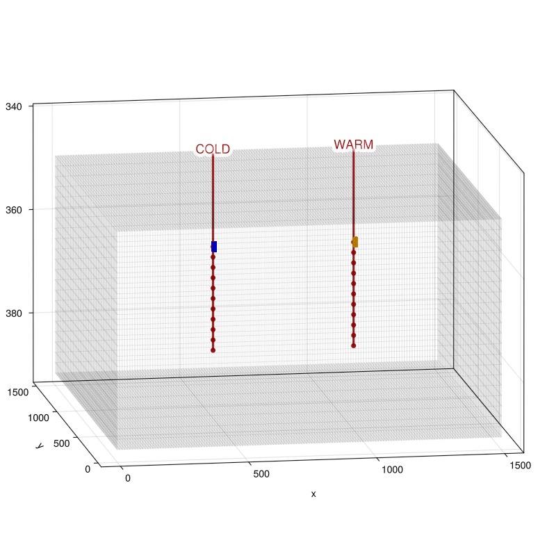
Plot the permeability
The model contains a high permeable aquifer layer in the middle of the model. The high permeable layer conducts the flow between the wells, and the low permeable layers above and below the aquifer layer conduct heat.
fig = Figure(size = (800, 800))
ax = Axis3(fig[1, 1], zreversed = true, azimuth = 4.55, elevation = 0.2)
for (wname, w) in get_model_wells(case)
    plot_well!(ax, G, w)
end
plt = plot_cell_data!(ax, G, reservoir[:permeability][1, :]./si_unit(:darcy),
    shading = NoShading,
    colormap = :thermal
)
Colorbar(fig[2, 1], plt, label = "Horizontal permeability (darcy)", vertical = false)
fig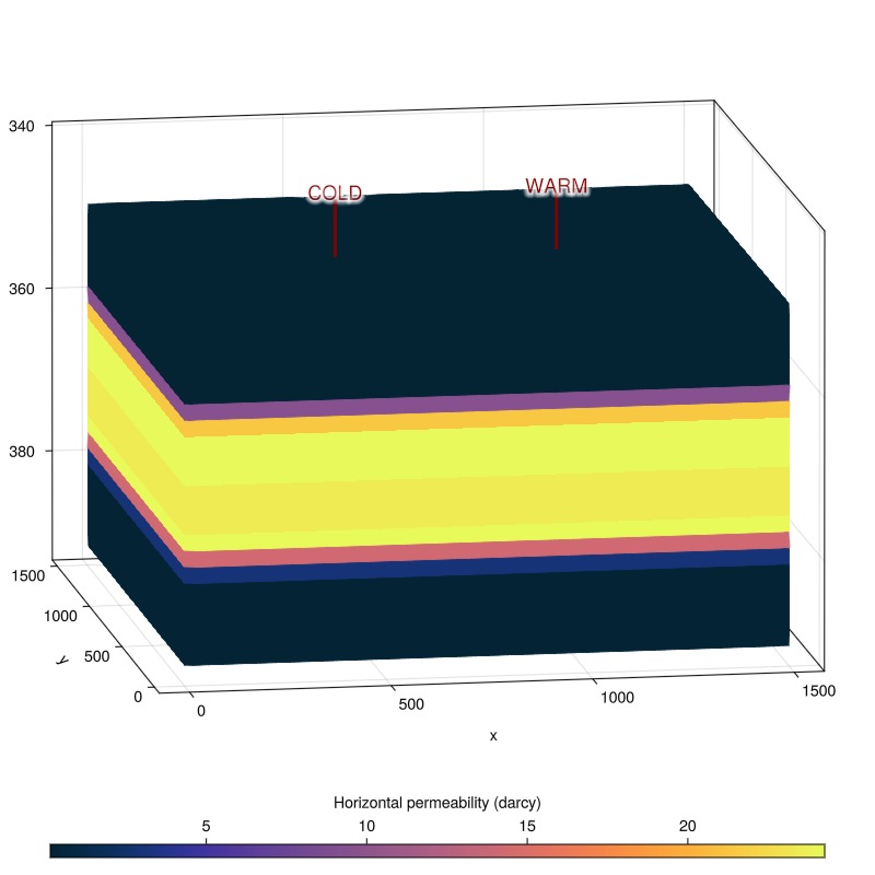
Plot the water rate in the wells
The water rate in the wells is shown below. The well rates are mirrored in that the cold well injects the same amount of water as the warm well produces and vice versa. Initially, the warm well injects water and the cold well produces to maintain aquifer pressure. Later on, the warm well produces warm water and the cold well injects utilized cold water at a slightly higher temperature than that of the reservoir to balance the pressure.
day = si_unit(:day)
t_jutul = t_seconds./day
wrat_cold = ws[:COLD][:wrat]*day
wrat_warm = ws[:WARM][:wrat]*day
fig = Figure()
ax = Axis(fig[1, 1], xlabel = "Time elapsed (days)", ylabel = "Water rate (m³/day)", title = "Water rate in wells (positive = injection)")
lines!(ax, t_jutul, wrat_cold, label = "COLD well", color = :blue)
lines!(ax, t_jutul, wrat_warm, label = "WARM well", color = :orange)
axislegend(position = :ct)
fig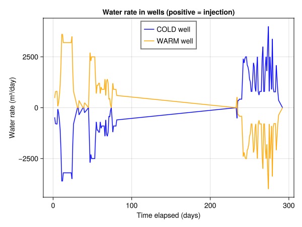
Plot the final temperature in the reservoir
We see the final temperature distribution in the reservoir. The regions near both wells are warmer than the rest of the reservoir, with the hot well being the warmest.
fig = Figure(size = (800, 800))
ax = Axis3(fig[1, 1], zreversed = true, azimuth = 4.55, elevation = 0.2)
for (wname, w) in get_model_wells(case)
    plot_well!(ax, G, w)
end
Jutul.plot_mesh_edges!(ax, G, alpha = 0.1)
temp = states[end][:Temperature] .- 273.15
plt = plot_cell_data!(ax, G, temp,
    colormap = :thermal,
    cells = findall(x -> x > 18, temp),
    transparency = true,
    shading = NoShading
)
Colorbar(fig[2, 1], plt, label = "Temperature (°C)", vertical = false)
fig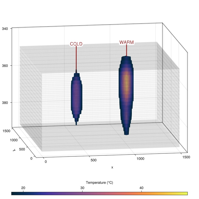
Plot the temperature near the warm well and compare to E300
We compare the temperature in cells close to the warm well in JutulDarcy and the same case simulated in E300, demonstrating excellent agreement.
warm1 = map(x -> x[:Temperature][cell_warm1] - 273.15, states)
warm2 = map(x -> x[:Temperature][cell_warm2] - 273.15, states)

t_e300 = cdata[:, 1]
warm1_e300 = cdata[:, 2]
warm2_e300 = cdata[:, 3]

fig = Figure()
ax = Axis(fig[1, 1], xlabel = "Time elapsed (days)", ylabel = "Temperature", title = "Temperature in cells close to warm well")
lines!(ax, t_jutul, warm1, label = "JutulDarcy, cell (105,75,6)", color = :orange)
lines!(ax, t_e300, warm1_e300, label = "E300, cell (105,75,6)", linestyle = :dash, linewidth = 3, color = :orange)

lines!(ax, t_jutul, warm2, label = "JutulDarcy, cell (106,75,6)", color = :blue)
lines!(ax, t_e300, warm2_e300, label = "E300, cell (106,75,6)", linestyle = :dash, linewidth = 3, color = :blue)
axislegend(position = :cb)
fig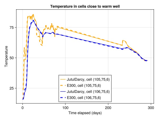
Plot the temperature near the cold well and compare
We note a similar match between the solvers near the cold well.
cold1 = map(x -> x[:Temperature][cell_cold1] - 273.15, states)
cold2 = map(x -> x[:Temperature][cell_cold2] - 273.15, states)

t_e300 = cdata[:, 1]
cold1_e300 = cdata[:, 4]
cold2_e300 = cdata[:, 5]

fig = Figure()
ax = Axis(fig[1, 1], xlabel = "Time elapsed (days)", ylabel = "Temperature", title = "Temperature in cells close to warm well")
lines!(ax, t_jutul, cold1, label = "JutulDarcy, cell (50,75,6)", color = :orange)
lines!(ax, t_e300, cold1_e300, label = "E300, cell (50,75,6)", linestyle = :dash, linewidth = 3, color = :orange)
lines!(ax, t_jutul, cold2, label = "JutulDarcy, cell (51,75,6)", color = :blue)
lines!(ax, t_e300, cold2_e300, label = "E300, cell (51,75,6)", linestyle = :dash, linewidth = 3, color = :blue)
axislegend(position = :ct)
fig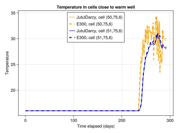
Plot the well temperatures
Finally, we compare the reported temperatures in the wells between JutulDarcy and E300. These values are a mix of prescribed conditions (during injection) and the solution values (during production).
t_well_e300 = wdata[:, 1]
warm_e300 = wdata[:, 2]
warm_jutul = ws[:WARM][:temperature] .- 273.15
cold_e300 = wdata[:, 3]
cold_jutul = ws[:COLD][:temperature] .- 273.15

fig = Figure()
ax = Axis(fig[1, 1], xlabel = "Time elapsed (days)", ylabel = "Temperature (°C)", title = "Well temperatures")
lines!(ax, t_jutul, warm_jutul, label = "JutulDarcy, WARM", color = :orange)
lines!(ax, t_well_e300, warm_e300, label = "E300, WARM", linestyle = :dash, linewidth = 3, color = :orange)
lines!(ax, t_jutul, cold_jutul, label = "JutulDarcy, COLD", color = :blue)
lines!(ax, t_well_e300, cold_e300, label = "E300, COLD", linestyle = :dash, linewidth = 3, color = :blue)
axislegend(position = :cb)
fig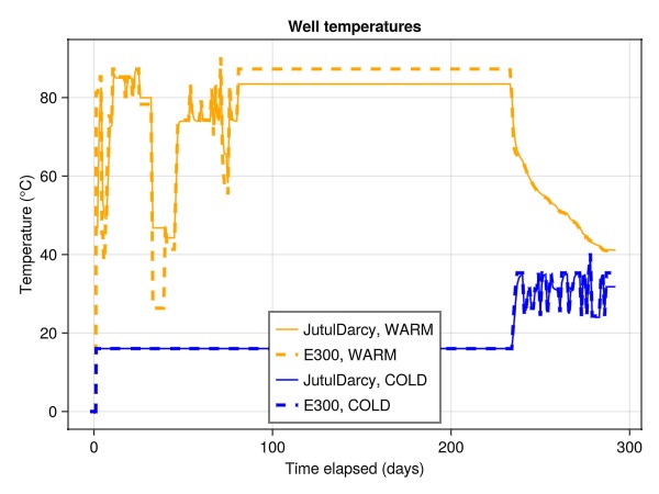
Plot the total energy in the reservoir
We plot the total energy in the reservoir relative to the initial condition by summing up the thermal energy in all cells at the initial state and using this as the baseline. The total energy in the reservoir matches the injected and produced energy, as there are no open boundary conditions.
E0 = sum(states[1][:TotalThermalEnergy])
energy = map(x -> sum(x[:TotalThermalEnergy]) - E0, states)
lines(t_jutul, energy, axis = (xlabel = "Time elapsed (days)", ylabel = "Total energy (J)", title = "Total energy in reservoir relative to initial condition"))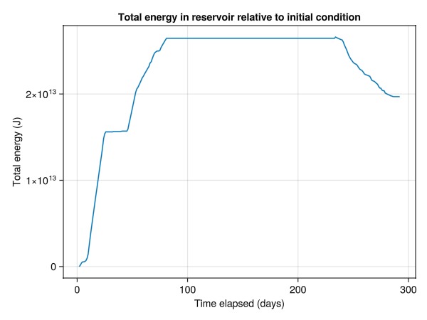
Plot the reservoir in the interactive viewer
If you are running this example yourself, you can launch an interactive viewer and explore the evolution of the model.
plot_reservoir(case, states, key = :Pressure, step = 100)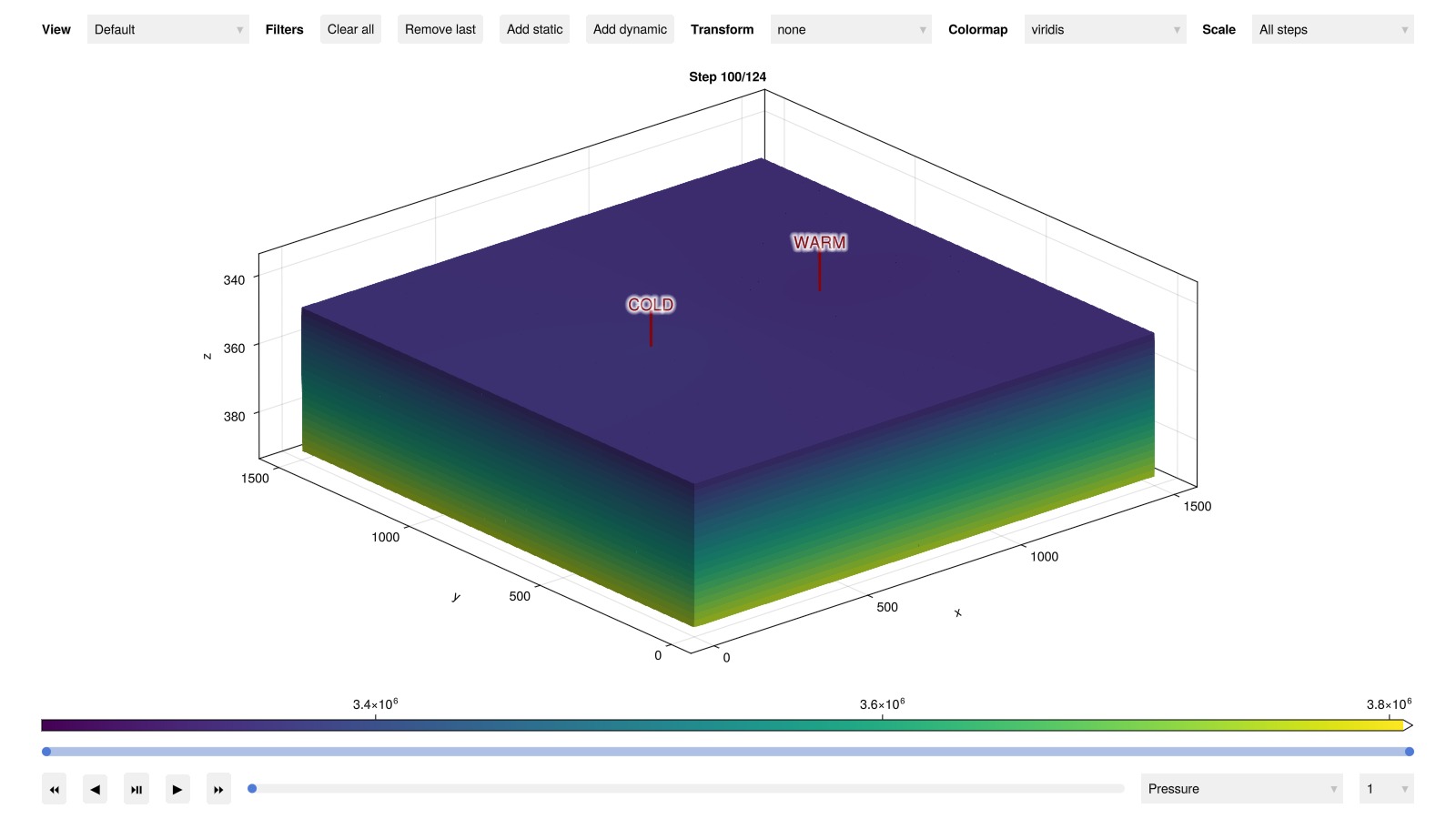
Example on GitHub
If you would like to run this example yourself, it can be downloaded from the JutulDarcy.jl GitHub repository as a script
This example took 546.468619081 seconds to complete.This page was generated using Literate.jl.