CO2 injection in saline aquifer with storage inventory

This example demonstrates a custom K-value compositional model for the injection of CO2 into a saline aquifer. The physical model for flow of CO2 is a realization of the description in 11th SPE Comparative Solutions Project. Simulation of CO2 can be challenging, and we load the HYPRE package to improve performance.

The model also has an option to run immiscible simulations with otherwise identical PVT behavior. This is often faster to run, but lacks the dissolution model present in the compositional version (i.e. no solubility of CO2 in brine, and no vaporization of water in the vapor phase).

use_immiscible = false
using Jutul, JutulDarcy
using HYPRE
using GLMakie
nx = 100
nz = 50
Darcy, bar, kg, meter, day, yr = si_units(:darcy, :bar, :kilogram, :meter, :day, :year)

(9.86923266716013e-13, 100000.0, 1.0, 1.0, 86400.0, 3.1556952e7)

Set up a 2D aquifer model

We set up a Cartesian mesh that is then transformed into an unstructured mesh. We can then modify the coordinates to create a domain with a undulating top surface. CO2 will flow along the top surface and the topography of the top surface has a large impact on where the CO2 migrates.

cart_dims = (nx, 1, nz)
physical_dims = (1000.0, 1.0, 50.0)
cart_mesh = CartesianMesh(cart_dims, physical_dims)
mesh = UnstructuredMesh(cart_mesh, z_is_depth = true)

points = mesh.node_points
for (i, pt) in enumerate(points)
    x, y, z = pt
    x_u = 2*π*x/1000.0
    w = 0.2
    dz = 0.05*x + 0.05*abs(x - 500.0)+ w*(30*sin(2.0*x_u) + 20*sin(5.0*x_u))
    points[i] = pt + [0, 0, dz]
end;

Find and plot cells intersected by a deviated injector well

We place a single injector well. This well was unfortunately not drilled completely straight, so we cannot directly use add_vertical_well based on logical indices. We instead define a matrix with three columns x, y, z that lie on the well trajectory and use utilities from Jutul to find the cells intersected by the trajectory.

import Jutul: find_enclosing_cells, plot_mesh_edges
trajectory = [
    645.0 0.5 75;    # First point
    660.0 0.5 85;    # Second point
    710.0 0.5 100.0  # Third point
]

wc = find_enclosing_cells(mesh, trajectory)

fig, ax, plt = plot_mesh_edges(mesh)
plot_mesh!(ax, mesh, cells = wc, transparency = true, alpha = 0.4)

MakieCore.Mesh{Tuple{GeometryBasics.Mesh{3, Float64, GeometryBasics.NgonFace{3, GeometryBasics.OffsetInteger{-1, UInt32}}, (:position, :normal), Tuple{Vector{GeometryBasics.Point{3, Float64}}, Vector{GeometryBasics.Vec{3, Float32}}}, Vector{GeometryBasics.NgonFace{3, GeometryBasics.OffsetInteger{-1, UInt32}}}}}}

View from the side

ax.azimuth[] = 1.5*π
ax.elevation[] = 0.0
lines!(ax, trajectory', color = :red)
fig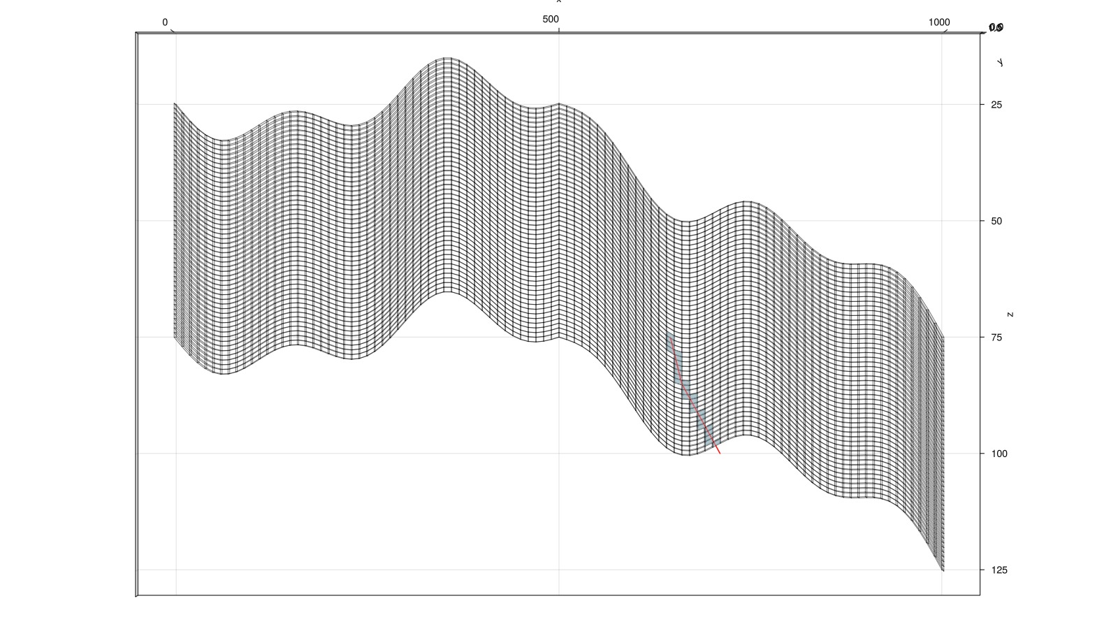

Define permeability and porosity

We loop over all cells and define three layered regions by the K index of each cell. We can then set a corresponding diagonal permeability tensor (3 values) and porosity (scalar) to introduce variation between the layers.

nc = number_of_cells(mesh)
perm = zeros(3, nc)
poro = fill(0.3, nc)
region = zeros(Int, nc)
for cell in 1:nc
    I, J, K = cell_ijk(mesh, cell)
    if K < 0.3*nz
        reg = 1
        permxy = 0.3*Darcy
        phi = 0.2
    elseif K < 0.7*nz
        reg = 2
        permxy = 1.2*Darcy
        phi = 0.35
    else
        reg = 3
        permxy = 0.1*Darcy
        phi = 0.1
    end
    permz = 0.5*permxy
    perm[1, cell] = perm[2, cell] = permxy
    perm[3, cell] = permz
    poro[cell] = phi
    region[cell] = reg
end

fig, ax, plt = plot_cell_data(mesh, poro)
fig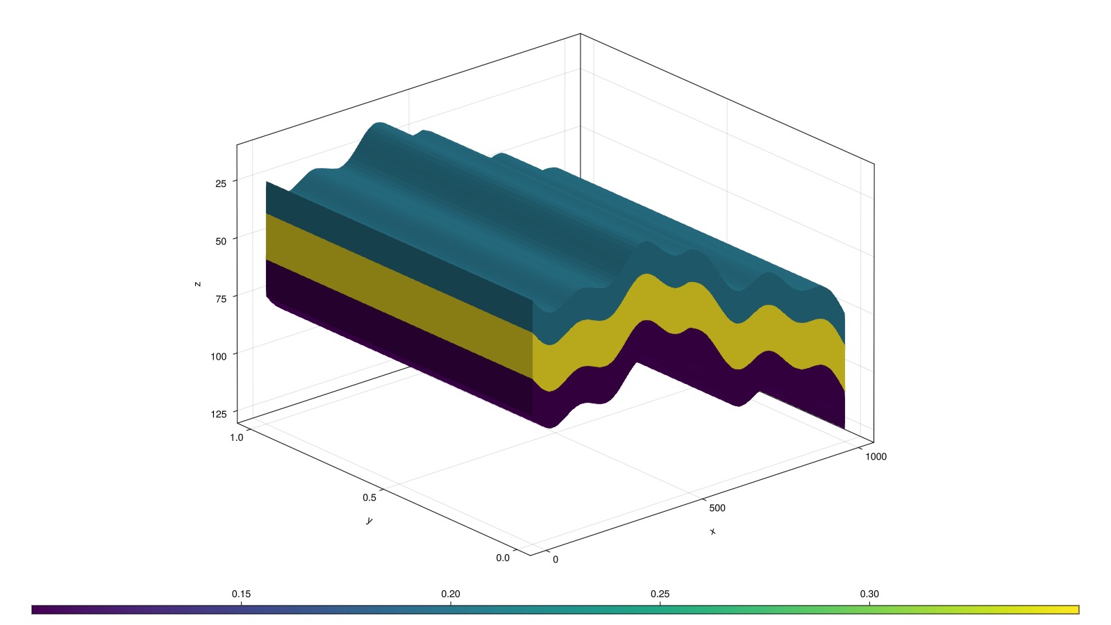

Set up simulation model

We set up a domain and a single injector. We pass the special :co2brine argument in place of the system to the reservoir model setup routine. This will automatically set up a compositional two-component CO2-H2O model with the appropriate functions for density, viscosity and miscibility.

Note that this model by default is isothermal, but we still need to specify a temperature when setting up the model. This is because the properties of CO2 strongly depend on temperature, even when thermal transport is not solved.

The model also accounts for a constant, reservoir-wide salinity. We input mole fractions of salts in the brine so that the solubilities, densities and viscosities for brine cells are corrected in the property model.

domain = reservoir_domain(mesh, permeability = perm, porosity = poro, temperature = convert_to_si(60.0, :Celsius))
Injector = setup_well(domain, wc, name = :Injector, simple_well = true)

if use_immiscible
    physics = :immiscible
else
    physics = :kvalue
end
model = setup_reservoir_model(domain, :co2brine,
    wells = Injector,
    extra_out = false,
    salt_names = ["NaCl", "KCl", "CaSO4", "CaCl2", "MgSO4", "MgCl2"],
    salt_mole_fractions = [0.01, 0.005, 0.005, 0.001, 0.0002, 1e-5],
    co2_physics = physics
);

Customize model by adding relative permeability with hysteresis

We define three relative permeability functions: kro(so) for the brine/liquid phase and krg(g) for both drainage and imbibition. Here we limit the hysteresis to only the non-wetting gas phase, but either combination of wetting or non-wetting hysteresis is supported.

Note that we import a few utilities from JutulDarcy that are not exported by default since hysteresis falls under advanced functionality.

import JutulDarcy: table_to_relperm, add_relperm_parameters!, brooks_corey_relperm
so = range(0, 1, 10)
krog_t = so.^2
krog = PhaseRelativePermeability(so, krog_t, label = :og)

PhaseRelativePermeability for og:
  .k: Internal representation: Jutul.LinearInterpolant{Vector{Float64}, Vector{Float64}, Missing}([-1.0e-16, 0.1111111111111111, 0.2222222222222222, 0.3333333333333333, 0.4444444444444444, 0.5555555555555556, 0.6666666666666666, 0.7777777777777778, 0.8888888888888887, 1.0], [0.0, 0.012345679012345678, 0.04938271604938271, 0.1111111111111111, 0.19753086419753085, 0.308641975308642, 0.4444444444444444, 0.6049382716049383, 0.7901234567901234, 1.0], missing)
  Connate saturation = 0.0
  Critical saturation = 0.0
  Maximum rel. perm = 1.0 at 1.0

Higher resolution for second table:

sg = range(0, 1, 50);

Evaluate Brooks-Corey to generate tables:

tab_krg_drain = brooks_corey_relperm.(sg, n = 2, residual = 0.1)
tab_krg_imb = brooks_corey_relperm.(sg, n = 3, residual = 0.25)

krg_drain  = PhaseRelativePermeability(sg, tab_krg_drain, label = :g)
krg_imb  = PhaseRelativePermeability(sg, tab_krg_imb, label = :g)

fig, ax, plt = lines(sg, tab_krg_drain, label = "krg drainage")
lines!(ax, sg, tab_krg_imb, label = "krg imbibition")
lines!(ax, 1 .- so, krog_t, label = "kro")
axislegend()
fig
# Define a relative permeability variable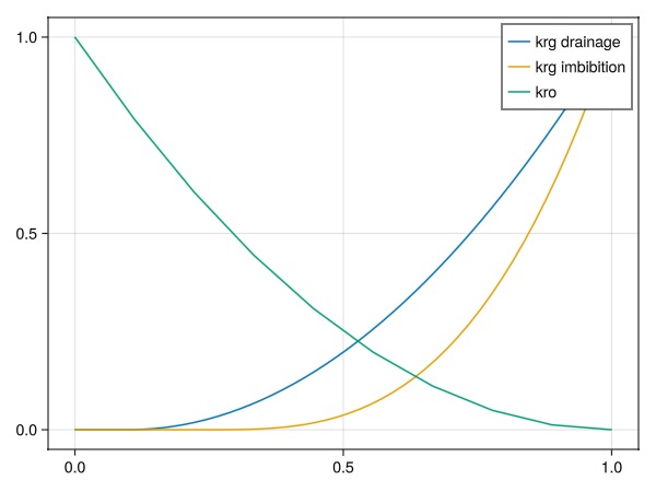

JutulDarcy uses type instances to define how different variables inside the simulation are evaluated. The ReservoirRelativePermeabilities type has support for up to three phases with w, ow, og and g relative permeabilities specified as a function of their respective phases. It also supports saturation regions.

Note: If regions are used, all drainage curves come first followed by equal number of imbibition curves. Since we only have a single (implicit) saturation region, the krg input should have two entries: One for drainage, and one for imbibition.

We also call add_relperm_parameters to the model. This makes sure that when hysteresis is enabled, we track maximum saturation for hysteresis in each reservoir cell.

import JutulDarcy: KilloughHysteresis, ReservoirRelativePermeabilities
krg = (krg_drain, krg_imb)
H_g = KilloughHysteresis() # Other options: CarlsonHysteresis, JargonHysteresis
relperm = ReservoirRelativePermeabilities(g = krg, og = krog, hysteresis_g = H_g)
replace_variables!(model, RelativePermeabilities = relperm)
add_relperm_parameters!(model);

Define approximate hydrostatic pressure and set up initial state

The initial pressure of the water-filled domain is assumed to be at hydrostatic equilibrium. If we use an immiscible model, we must provide the initial saturations. If we are using a compositional model, we should instead provide the overall mole fractions. Note that since both are fractions, and the CO2 model has correspondence between phase ordering and component ordering (i.e. solves for liquid and vapor, and H2O and CO2), we can use the same input value.

nc = number_of_cells(mesh)
p0 = zeros(nc)
depth = domain[:cell_centroids][3, :]
g = Jutul.gravity_constant
@. p0 = 160bar + depth*g*1000.0
fig, ax, plt = plot_cell_data(mesh, p0)
fig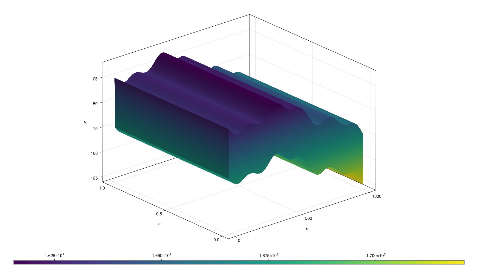

Set up initial state and parameters

if use_immiscible
    state0 = setup_reservoir_state(model,
        Pressure = p0,
        Saturations = [1.0, 0.0],
    )
else
    state0 = setup_reservoir_state(model,
        Pressure = p0,
        OverallMoleFractions = [1.0, 0.0],
    )
end
parameters = setup_parameters(model)

Dict{Symbol, Any} with 3 entries:
  :Injector  => Dict{Symbol, Any}(:FluidVolume=>[0.0630954], :WellIndicesTherma…
  :Reservoir => Dict{Symbol, Any}(:Transmissibilities=>[2.85521e-14, 2.87444e-1…
  :Facility  => Dict{Symbol, Any}()

Find the boundary and apply a constant pressureboundary condition

We find cells on the left and right boundary of the model and set a constant pressure boundary condition to represent a bounding aquifer that retains the initial pressure far away from injection.

boundary = Int[]
for cell in 1:nc
    I, J, K = cell_ijk(mesh, cell)
    if I == 1 || I == nx
        push!(boundary, cell)
    end
end
bc = flow_boundary_condition(boundary, domain, p0[boundary], fractional_flow = [1.0, 0.0])
println("Boundary condition added to $(length(bc)) cells.")

Boundary condition added to 100 cells.

Plot the model

plot_reservoir(model)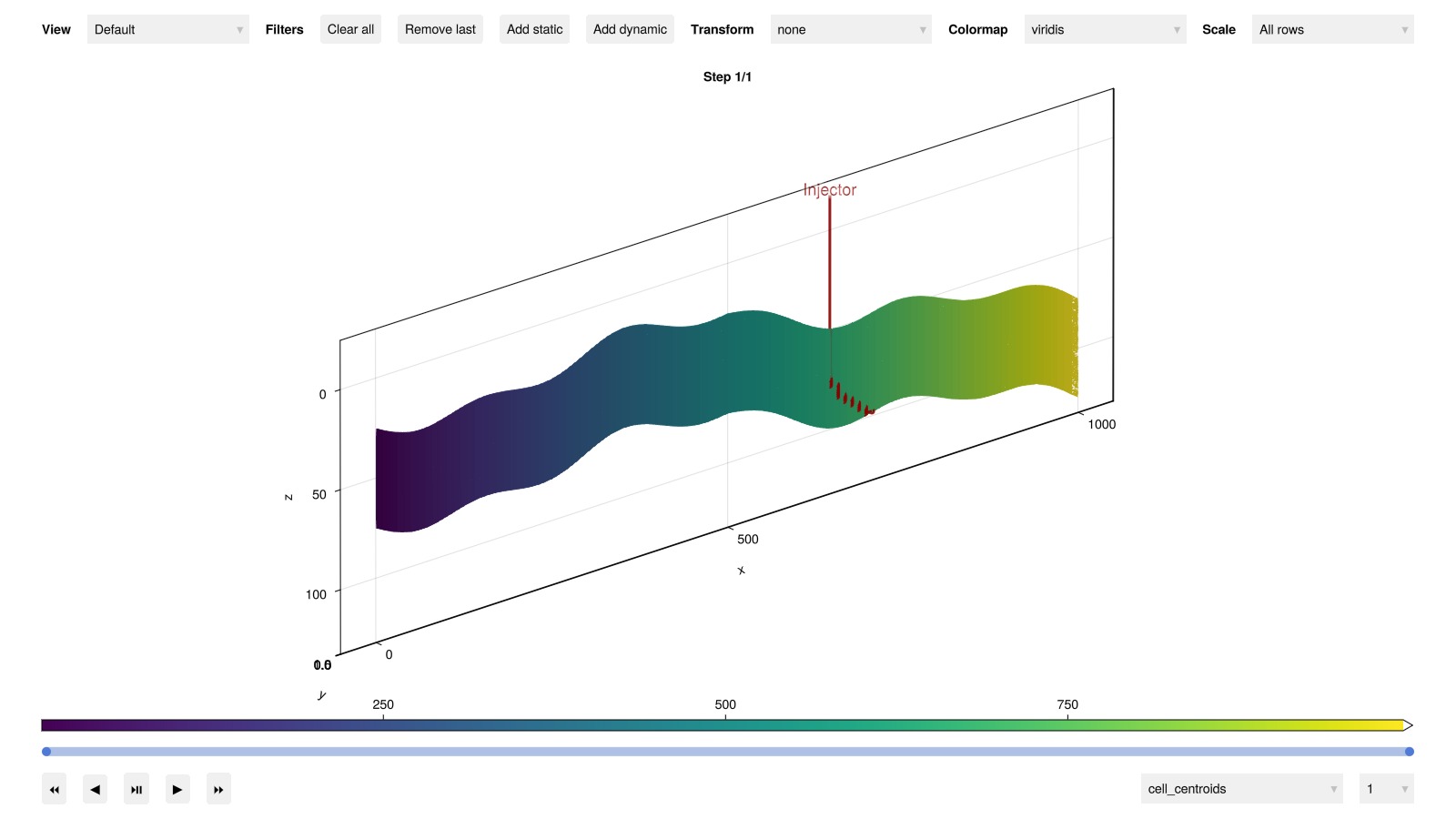

Set up schedule

We set up 25 years of injection and 475 years of migration where the well is shut. The density of the injector is set to 630 kg/m^3, which is roughly the density of CO2 at the in-situ conditions.

nstep = 25
nstep_shut = 475
dt_inject = fill(365.0day, nstep)
pv = pore_volume(model, parameters)
inj_rate = 0.075*sum(pv)/sum(dt_inject)

rate_target = TotalRateTarget(inj_rate)
I_ctrl = InjectorControl(rate_target, [0.0, 1.0],
    density = 630.0,
)

InjectorControl{TotalRateTarget{Float64}, Float64, Tuple{Tuple{Int64, Float64}}, Vector{Float64}, Missing, Missing}(TotalRateTarget with value 1.084474885844749e-6 [m^3/s], [0.0, 1.0], 630.0, ((1, 1.0),), 293.15, missing, 1.0, missing)

Set up forces for use in injection

controls = Dict(:Injector => I_ctrl)
forces_inject = setup_reservoir_forces(model, control = controls, bc = bc)

Dict{Symbol, Any} with 3 entries:
  :Injector  => (mask = nothing,)
  :Reservoir => (bc = FlowBoundaryCondition{Int64, Float64, Tuple{Float64, Floa…
  :Facility  => (control = Dict{Symbol, InjectorControl{TotalRateTarget{Float64…

Forces with shut wells

forces_shut = setup_reservoir_forces(model, bc = bc)
dt_shut = fill(365.0day, nstep_shut);

Combine the report steps and forces into vectors of equal length

dt = vcat(dt_inject, dt_shut)
forces = vcat(
    fill(forces_inject, nstep),
    fill(forces_shut, nstep_shut)
)
println("$nstep report steps with injection, $nstep_shut report steps with migration.")

25 report steps with injection, 475 report steps with migration.

Add some more outputs for plotting

rmodel = reservoir_model(model)
push!(rmodel.output_variables, :RelativePermeabilities)
push!(rmodel.output_variables, :PhaseViscosities)

9-element Vector{Symbol}:
 :Pressure
 :OverallMoleFractions
 :TotalMasses
 :LiquidMassFractions
 :VaporMassFractions
 :Saturations
 :PhaseMassDensities
 :RelativePermeabilities
 :PhaseViscosities

Simulate the schedule

We set a maximum internal time-step of 30 days to ensure smooth convergence and reduce numerical diffusion.

wd, states, t = simulate_reservoir(state0, model, dt,
    parameters = parameters,
    forces = forces,
    max_timestep = 90day
);

Jutul: Simulating 499 years, 34.86 weeks as 500 report steps
╭────────────────┬───────────┬────────────────┬──────────────╮
│ Iteration type │  Avg/step │   Avg/ministep │        Total │
│                │ 500 steps │ 2572 ministeps │     (wasted) │
├────────────────┼───────────┼────────────────┼──────────────┤
│ Newton         │      8.98 │        1.74572 │   4490 (375) │
│ Linearization  │    14.124 │        2.74572 │   7062 (400) │
│ Linear solver  │    39.442 │        7.66757 │ 19721 (1399) │
│ Precond apply  │    78.884 │        15.3351 │ 39442 (2798) │
╰────────────────┴───────────┴────────────────┴──────────────╯
╭───────────────┬─────────┬────────────┬─────────╮
│ Timing type   │    Each │   Relative │   Total │
│               │      ms │ Percentage │       s │
├───────────────┼─────────┼────────────┼─────────┤
│ Properties    │  1.7537 │    13.40 % │  7.8741 │
│ Equations     │  0.8855 │    10.64 % │  6.2536 │
│ Assembly      │  0.5930 │     7.13 % │  4.1877 │
│ Linear solve  │  0.6629 │     5.06 % │  2.9764 │
│ Linear setup  │  3.1367 │    23.96 % │ 14.0840 │
│ Precond apply │  0.3888 │    26.09 % │ 15.3338 │
│ Update        │  0.2012 │     1.54 % │  0.9033 │
│ Convergence   │  0.3854 │     4.63 % │  2.7215 │
│ Input/Output  │  0.0833 │     0.36 % │  0.2141 │
│ Other         │  0.9406 │     7.19 % │  4.2233 │
├───────────────┼─────────┼────────────┼─────────┤
│ Total         │ 13.0895 │   100.00 % │ 58.7719 │
╰───────────────┴─────────┴────────────┴─────────╯

Plot the CO2 mole fraction

We plot the overall CO2 mole fraction. We scale the color range to log10 to account for the fact that the mole fraction in cells made up of only the aqueous phase is much smaller than that of cells with only the gaseous phase, where there is almost just CO2.

The aquifer gives some degree of passive flow through the domain, ensuring that much of the dissolved CO2 will leave the reservoir by the end of the injection period.

using GLMakie
function plot_co2!(fig, ix, x, title = "")
    ax = Axis3(fig[ix, 1],
        zreversed = true,
        azimuth = -0.51π,
        elevation = 0.05,
        aspect = (1.0, 1.0, 0.3),
        title = title)
    plt = plot_cell_data!(ax, mesh, x, colormap = :seaborn_icefire_gradient)
    Colorbar(fig[ix, 2], plt)
end
fig = Figure(size = (900, 1200))
for (i, step) in enumerate([5, nstep, nstep + Int(floor(nstep_shut/2)), nstep+nstep_shut])
    if use_immiscible
        plot_co2!(fig, i, states[step][:Saturations][2, :], "CO2 plume saturation at report step $step/$(nstep+nstep_shut)")
    else
        plot_co2!(fig, i, log10.(states[step][:OverallMoleFractions][2, :]), "log10 of CO2 mole fraction at report step $step/$(nstep+nstep_shut)")
    end
end
fig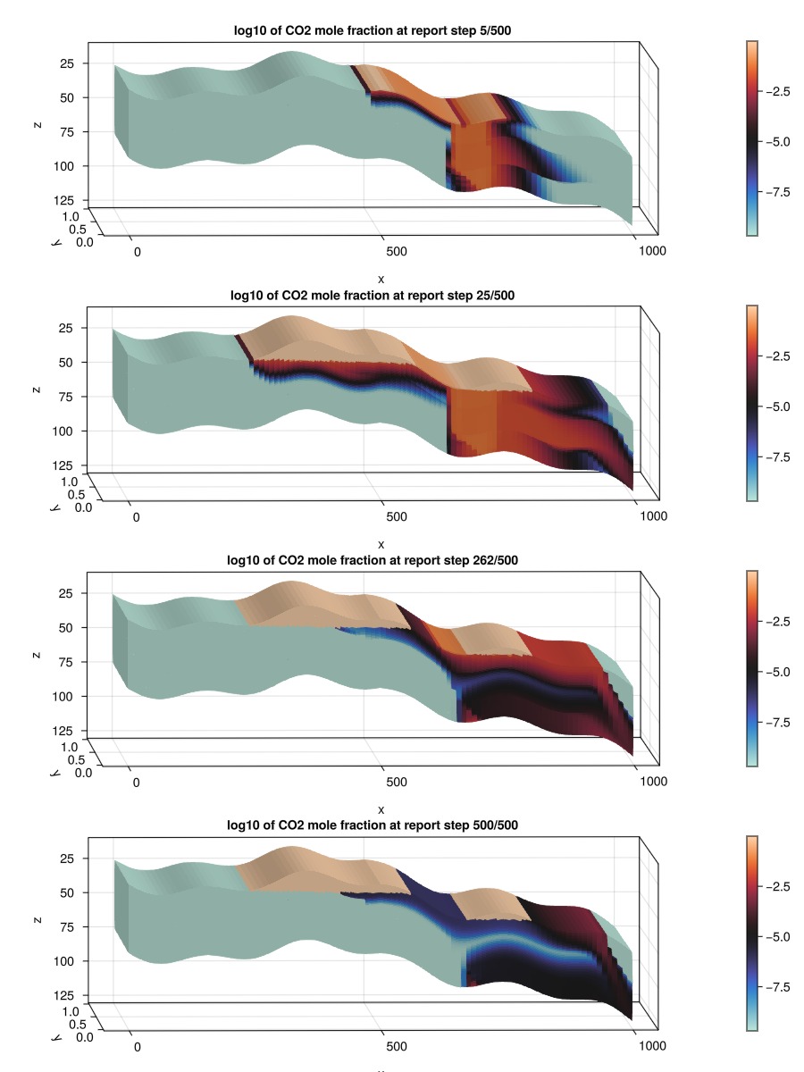

Plot all relative permeabilities for all time-steps

We can plot all relative permeability evaluations. This both verifies that the hysteresis model is active, but also gives an indication to how many cells are exhibiting imbibition during the simulation.

kro_val = Float64[]
krg_val = Float64[]
sg_val = Float64[]
for state in states
    kr_state = state[:RelativePermeabilities]
    s_state = state[:Saturations]
    for c in 1:nc
        push!(kro_val, kr_state[1, c])
        push!(krg_val, kr_state[2, c])
        push!(sg_val, s_state[2, c])
    end
end

fig = Figure()
ax = Axis(fig[1, 1], title = "Relative permeability during simulation")
fig, ax, plt = scatter(sg_val, kro_val, label = "kro", alpha = 0.3)
scatter!(ax, sg_val, krg_val, label = "krg", alpha = 0.3)
axislegend()
fig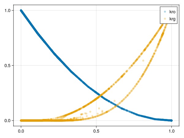

Plot result in interactive viewer

If you have interactive plotting available, you can explore the results yourself.

plot_reservoir(model, states)
# Calculate and display inventory of CO2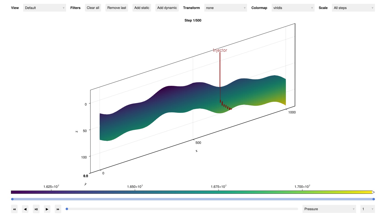

We can classify and plot the status of the CO2 in the reservoir. We use a fairly standard classification where CO2 is divided into:

• dissolved CO2 (dissolution trapping)

• residual CO2 (immobile due to zero relative permeability, residual trapping)

• mobile CO2 (mobile but still inside domain)

• outside domain (left the simulation model and migrated outside model)

We also note that some of the mobile CO2 could be considered to be structurally trapped, but this is not classified in our inventory.

inventory = co2_inventory(model, wd, states, t)
JutulDarcy.plot_co2_inventory(t, inventory)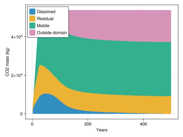

Pick a region to investigate the CO2

We can also specify a region to the CO2 inventory. This will introduce additional categories to distinguish between outside and inside the region of interest.

cells = findall(region .== 2)
inventory = co2_inventory(model, wd, states, t, cells = cells)
JutulDarcy.plot_co2_inventory(t, inventory)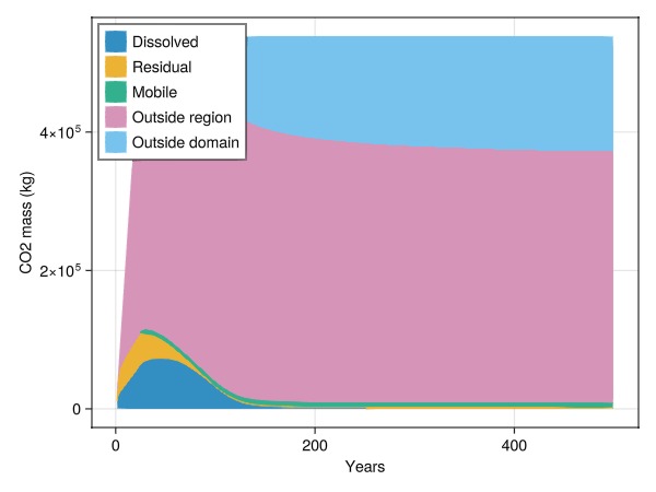

Define a region of interest using geometry

Another alternative to determine a region of interest is to use geometry. We pick all cells within an ellipsoid a bit away from the injection point.

is_inside = fill(false, nc)
centers = domain[:cell_centroids]
for cell in 1:nc
    x, y, z = centers[:, cell]
    is_inside[cell] = sqrt((x - 720.0)^2 + 20*(z-70.0)^2) < 75
end
fig, ax, plt = plot_cell_data(mesh, is_inside)
fig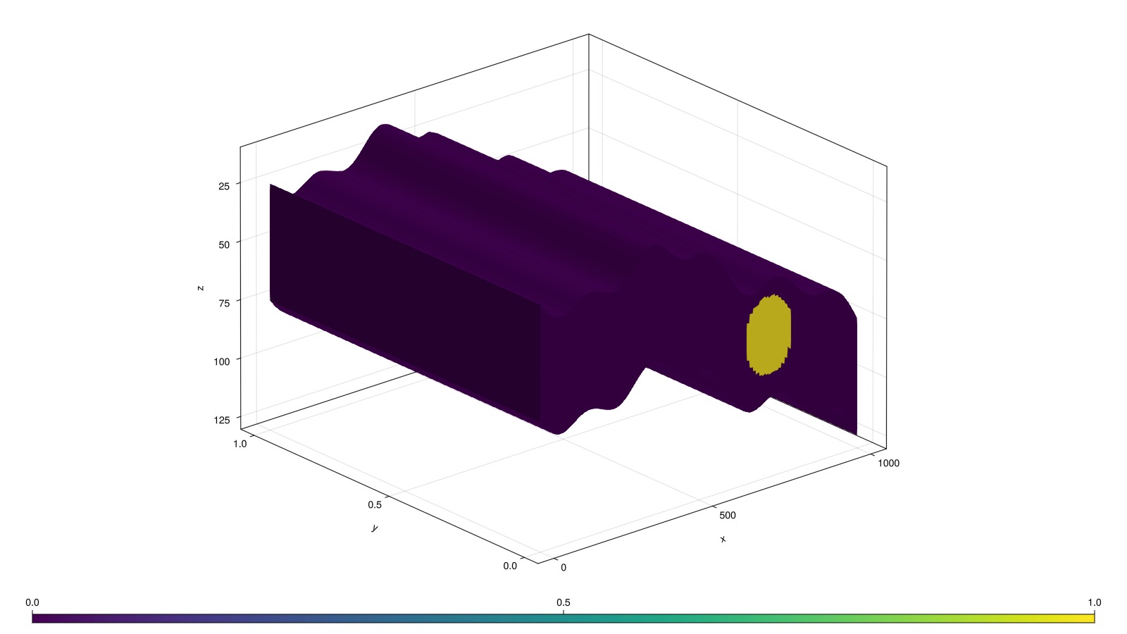

Plot inventory in ellipsoid

Note that a small mobile dip can be seen when free CO2 passes through this region.

inventory = co2_inventory(model, wd, states, t, cells = findall(is_inside))
JutulDarcy.plot_co2_inventory(t, inventory)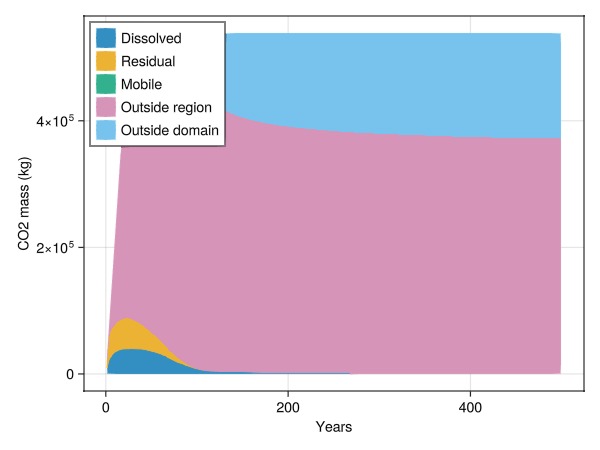

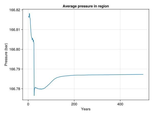
Plot the average pressure in the ellipsoid region

Now that we know what cells are within the region of interest, we can easily apply a function over all time-steps to figure out what the average pressure value was.

using Statistics
p_avg = map(
    state -> mean(state[:Pressure][is_inside])./bar,
    states
)
lines(t./yr, p_avg,
    axis = (
        title = "Average pressure in region",
        xlabel = "Years", ylabel = "Pressure (bar)"
    )
)

Make a composite plot to correlate CO2 mass in region with spatial distribution

We create a pair of plots that combine both 2D and 3D plots to simultaneously show the ellipsoid, the mass of CO2 in that region for a specific step, and the time series of the CO2 in the same region.

stepno = 30
co2_mass_in_region = map(
    state -> sum(state[:TotalMasses][2, is_inside])/1e3,
    states
)
fig = Figure(size = (1200, 600))
ax1 = Axis(fig[1, 1],
    title = "Mass of CO2 in region",
    xlabel = "Years",
    ylabel = "Tonnes CO2"
)
lines!(ax1, t./yr, co2_mass_in_region)
scatter!(ax1, t[stepno]./yr, co2_mass_in_region[stepno], markersize = 12, color = :red)
ax2 = Axis3(fig[1, 2], zreversed = true)
plot_cell_data!(ax2, mesh, states[stepno][:TotalMasses][2, :])
plot_mesh!(ax2, mesh, cells = findall(is_inside), alpha = 0.5)
ax2.azimuth[] = 1.5*π
ax2.elevation[] = 0.0
fig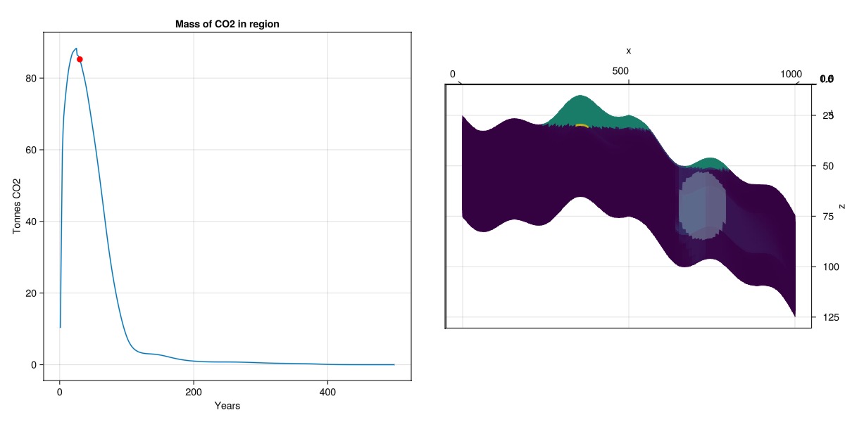

Example on GitHub

If you would like to run this example yourself, it can be downloaded from the JutulDarcy.jl GitHub repository as a script, or as a Jupyter Notebook

This example took 1185.946525581 seconds to complete.

---

This page was generated using Literate.jl.