Gradient-based matching of parameters against observations

We create a simple test problem: A 1D nonlinear displacement. The observations are generated by solving the same problem with the true parameters. We then match the parameters against the observations using a different starting guess for the parameters, but otherwise the same physical description of the system.

This example uses the numerical parameter optimization framework in Jutul for model calibration. Later on, the high-level interface for optimization is also demonstrated.

using Jutul
using JutulDarcy
using LinearAlgebra
using GLMakie

Define a setup function

irate = 10.0
function setup_bl(;nc = 100, time = 1.0, nstep = 100, poro = 0.1, perm = 0.1*si_unit(:darcy))
    T = time
    tstep = repeat([T/nstep], nstep)
    G = get_1d_reservoir(nc, poro = poro, perm = perm)
    nc = number_of_cells(G)

    bar = 1e5
    p0 = 1000*bar
    sys = ImmiscibleSystem((LiquidPhase(), VaporPhase()))
    model = SimulationModel(G, sys)
    model.primary_variables[:Pressure] = Pressure(minimum = -Inf, max_rel = nothing)
    kr = BrooksCoreyRelativePermeabilities(sys, [2.0, 2.0])
    replace_variables!(model, RelativePermeabilities = kr)
    tot_time = sum(tstep)

    parameters = setup_parameters(model, PhaseViscosities = [1e-3, 5e-3]) # 1 and 5 cP
    state0 = setup_state(model, Pressure = p0, Saturations = [0.0, 1.0])

    src  = [SourceTerm(1, irate, fractional_flow = [1.0-1e-3, 1e-3]),
            SourceTerm(nc, -irate, fractional_flow = [1.0, 0.0])]
    forces = setup_forces(model, sources = src)

    return JutulCase(model, tstep, forces, state0 = state0, parameters = parameters)
end

setup_bl (generic function with 1 method)

Number of cells and time-steps

N = 100
Nt = 100
poro_ref = 0.1
perm_ref = 0.1*si_unit(:darcy)

9.86923266716013e-14

Set up and simulate reference

case_ref = setup_bl(nc = N, nstep = Nt, poro = poro_ref, perm = perm_ref)
states_ref, = simulate(case_ref);

Jutul: Simulating 1 second as 100 report steps
╭────────────────┬───────────┬───────────────┬──────────╮
│ Iteration type │  Avg/step │  Avg/ministep │    Total │
│                │ 100 steps │ 100 ministeps │ (wasted) │
├────────────────┼───────────┼───────────────┼──────────┤
│ Newton         │      1.07 │          1.07 │  107 (0) │
│ Linearization  │      2.07 │          2.07 │  207 (0) │
│ Linear solver  │      1.07 │          1.07 │  107 (0) │
│ Precond apply  │       0.0 │           0.0 │    0 (0) │
╰────────────────┴───────────┴───────────────┴──────────╯
╭───────────────┬─────────┬────────────┬────────╮
│ Timing type   │    Each │   Relative │  Total │
│               │      ms │ Percentage │      s │
├───────────────┼─────────┼────────────┼────────┤
│ Properties    │  0.0165 │     0.04 % │ 0.0018 │
│ Equations     │  2.4352 │    10.50 % │ 0.5041 │
│ Assembly      │  1.7659 │     7.61 % │ 0.3655 │
│ Linear solve  │ 15.1420 │    33.75 % │ 1.6202 │
│ Linear setup  │  0.0000 │     0.00 % │ 0.0000 │
│ Precond apply │  0.0000 │     0.00 % │ 0.0000 │
│ Update        │  3.1982 │     7.13 % │ 0.3422 │
│ Convergence   │  2.4167 │    10.42 % │ 0.5003 │
│ Input/Output  │  0.4196 │     0.87 % │ 0.0420 │
│ Other         │ 13.3134 │    29.67 % │ 1.4245 │
├───────────────┼─────────┼────────────┼────────┤
│ Total         │ 44.8648 │   100.00 % │ 4.8005 │
╰───────────────┴─────────┴────────────┴────────╯

Set up another case where the porosity is different

case_dporo = setup_bl(nc = N, nstep = Nt, poro = 2*poro_ref, perm = 1.0*perm_ref)
states, rep = simulate(case_dporo);

Jutul: Simulating 1 second as 100 report steps
╭────────────────┬───────────┬───────────────┬──────────╮
│ Iteration type │  Avg/step │  Avg/ministep │    Total │
│                │ 100 steps │ 100 ministeps │ (wasted) │
├────────────────┼───────────┼───────────────┼──────────┤
│ Newton         │      1.01 │          1.01 │  101 (0) │
│ Linearization  │      2.01 │          2.01 │  201 (0) │
│ Linear solver  │      1.01 │          1.01 │  101 (0) │
│ Precond apply  │       0.0 │           0.0 │    0 (0) │
╰────────────────┴───────────┴───────────────┴──────────╯
╭───────────────┬──────────┬────────────┬──────────╮
│ Timing type   │     Each │   Relative │    Total │
│               │       μs │ Percentage │       ms │
├───────────────┼──────────┼────────────┼──────────┤
│ Properties    │  16.0342 │     1.61 % │   1.6195 │
│ Equations     │  19.6337 │     3.93 % │   3.9464 │
│ Assembly      │   6.1926 │     1.24 % │   1.2447 │
│ Linear solve  │ 835.1572 │    83.91 % │  84.3509 │
│ Linear setup  │   0.0000 │     0.00 % │   0.0000 │
│ Precond apply │   0.0000 │     0.00 % │   0.0000 │
│ Update        │  11.7286 │     1.18 % │   1.1846 │
│ Convergence   │  11.1627 │     2.23 % │   2.2437 │
│ Input/Output  │  10.2026 │     1.01 % │   1.0203 │
│ Other         │  48.6796 │     4.89 % │   4.9166 │
├───────────────┼──────────┼────────────┼──────────┤
│ Total         │ 995.3131 │   100.00 % │ 100.5266 │
╰───────────────┴──────────┴────────────┴──────────╯

Plot the results

fig = Figure()
ax = Axis(fig[1, 1], title = "Saturation")
lines!(ax, states_ref[end][:Saturations][1, :], label = "Reference")
lines!(ax, states[end][:Saturations][1, :], label = "Initial guess")
axislegend(ax)
ax = Axis(fig[1, 2], title = "Pressure")
lines!(ax, states_ref[end][:Pressure], label = "Reference")
lines!(ax, states[end][:Pressure], label = "Initial guess")
axislegend(ax)
fig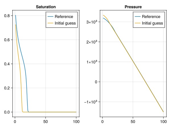

Define objective function

Define objective as mismatch between water saturation in current state and reference state. The objective function is currently a sum over all time steps. We implement a function for one term of this sum.

step_times = cumsum(case_ref.dt)
function saturation_mismatch(m, state, dt, step_info, forces)
    t = step_info[:time] + dt
    step_no = findmin(x -> abs(x - t), step_times)[2]
    state_ref = states_ref[step_no]
    fld = :Saturations
    val = state[fld]
    ref = state_ref[fld]
    err = 0
    for i in axes(val, 2)
        err += (val[1, i] - ref[1, i])^2
    end
    return dt*err
end
forces = case_ref.forces
dt = case_ref.dt
model = case_ref.model
@assert Jutul.evaluate_objective(saturation_mismatch, model, states_ref, dt, forces) == 0.0
@assert Jutul.evaluate_objective(saturation_mismatch, model, states, dt, forces) > 0.0

Set up a configuration for the optimization

The optimization code enables all parameters for optimization by default, with relative box limits 0.1 and 10 specified here. If use_scaling is enabled the variables in the optimization are scaled so that their actual limits are approximately box limits.

We are not interested in matching gravity effects or viscosity here. Transmissibilities are derived from permeability and varies significantly. We can set log scaling to get a better conditioned optimization system, without changing the limits or the result.

cfg = optimization_config(case_dporo, use_scaling = true, rel_min = 0.1, rel_max = 10)
for (ki, vi) in cfg
    if ki in [:TwoPointGravityDifference, :PhaseViscosities, :Transmissibilities]
        vi[:active] = false
    end
end
print_obj = 100;

Set up parameter optimization

This gives us a set of function handles together with initial guess and limits. Generally calling either of the functions will mutate the data Dict. The options are: F_o(x) -> evaluate objective dF_o(dFdx, x) -> evaluate gradient of objective, mutating dFdx (may trigger evaluation of F_o) F_and_dF(F, dFdx, x) -> evaluate F and/or dF. Value of nothing will mean that the corresponding entry is skipped.

F_o, dF_o, F_and_dF, x0, lims, data = setup_parameter_optimization(case_dporo, saturation_mismatch, cfg, print = print_obj, param_obj = true);
F_initial = F_o(x0)
dF_initial = dF_o(similar(x0), x0)
@info "Initial objective: $F_initial, gradient norm $(norm(dF_initial))"

Parameters for model
┌─────────────┬────────┬─────┬─────────┬─────────────────┬─────────────┬────────────────┬─────────┬───────────┐
│        Name │ Entity │   N │   Scale │     Abs. limits │ Rel. limits │         Limits │ Lumping │      Type │
├─────────────┼────────┼─────┼─────────┼─────────────────┼─────────────┼────────────────┼─────────┼───────────┤
│ FluidVolume │  Cells │ 100 │ default │ [2.22e-16, Inf] │   [0.1, 10] │ [0.0002, 0.02] │       - │ parameter │
└─────────────┴────────┴─────┴─────────┴─────────────────┴─────────────┴────────────────┴─────────┴───────────┘
[ Info: Initial objective: 0.6770524662003109, gradient norm 4.126665648044461

Link to an optimizer package

We use Optim.jl but the interface is general enough that e.g. LBFGSB.jl can easily be swapped in.

LBFGS is a good choice for this problem, as Jutul provides sensitivities via adjoints that are inexpensive to compute.

import Optim
lower, upper = lims
inner_optimizer = Optim.LBFGS()
opts = Optim.Options(store_trace = true, show_trace = true, time_limit = 30)
results = Optim.optimize(Optim.only_fg!(F_and_dF), lower, upper, x0, Optim.Fminbox(inner_optimizer), opts)
x = results.minimizer
display(results)
F_final = F_o(x)

0.00011277009530714113

Compute the solution using the tuned parameters found in x.

parameters_t = deepcopy(case_dporo.parameters)
devectorize_variables!(parameters_t, model, x, data[:mapper], config = data[:config])
x_truth = vectorize_variables(case_ref.model, case_ref.parameters, data[:mapper], config = data[:config])
states_tuned, = simulate(case_dporo.state0, case_dporo.model, case_dporo.dt, parameters = parameters_t, forces = case_dporo.forces);

Jutul: Simulating 1 second as 100 report steps
╭────────────────┬───────────┬───────────────┬──────────╮
│ Iteration type │  Avg/step │  Avg/ministep │    Total │
│                │ 100 steps │ 100 ministeps │ (wasted) │
├────────────────┼───────────┼───────────────┼──────────┤
│ Newton         │      1.07 │          1.07 │  107 (0) │
│ Linearization  │      2.07 │          2.07 │  207 (0) │
│ Linear solver  │      1.07 │          1.07 │  107 (0) │
│ Precond apply  │       0.0 │           0.0 │    0 (0) │
╰────────────────┴───────────┴───────────────┴──────────╯
╭───────────────┬──────────┬────────────┬─────────╮
│ Timing type   │     Each │   Relative │   Total │
│               │       μs │ Percentage │      ms │
├───────────────┼──────────┼────────────┼─────────┤
│ Properties    │  14.9665 │     4.43 % │  1.6014 │
│ Equations     │  19.1136 │    10.94 % │  3.9565 │
│ Assembly      │   6.2835 │     3.60 % │  1.3007 │
│ Linear solve  │ 191.2881 │    56.60 % │ 20.4678 │
│ Linear setup  │   0.0000 │     0.00 % │  0.0000 │
│ Precond apply │   0.0000 │     0.00 % │  0.0000 │
│ Update        │  10.1985 │     3.02 % │  1.0912 │
│ Convergence   │  10.2269 │     5.85 % │  2.1170 │
│ Input/Output  │   9.1783 │     2.54 % │  0.9178 │
│ Other         │  44.0282 │    13.03 % │  4.7110 │
├───────────────┼──────────┼────────────┼─────────┤
│ Total         │ 337.9766 │   100.00 % │ 36.1635 │
╰───────────────┴──────────┴────────────┴─────────╯

Plot final parameter spread

@info "Final residual $F_final (down from $F_initial)"
fig = Figure()
ax1 = Axis(fig[1, 1], title = "Scaled parameters", ylabel = "Value")
scatter!(ax1, x, label = "Final X")
scatter!(ax1, x0, label = "Initial X")
scatter!(ax1, x_truth, label = "Reference X")
lines!(ax1, lower, label = "Lower bound")
lines!(ax1, upper, label = "Upper bound")
axislegend()
fig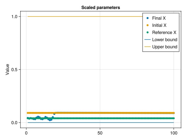

Plot the final solutions.

Note that we only match saturations - so any match in pressure is not guaranteed.

fig = Figure()
ax = Axis(fig[1, 1], title = "Saturation")
lines!(ax, states_ref[end][:Saturations][1, :], label = "Reference")
lines!(ax, states[end][:Saturations][1, :], label = "Initial guess")
lines!(ax, states_tuned[end][:Saturations][1, :], label = "Tuned")

axislegend(ax)
ax = Axis(fig[1, 2], title = "Pressure")
lines!(ax, states_ref[end][:Pressure], label = "Reference")
lines!(ax, states[end][:Pressure], label = "Initial guess")
lines!(ax, states_tuned[end][:Pressure], label = "Tuned")
axislegend(ax)
fig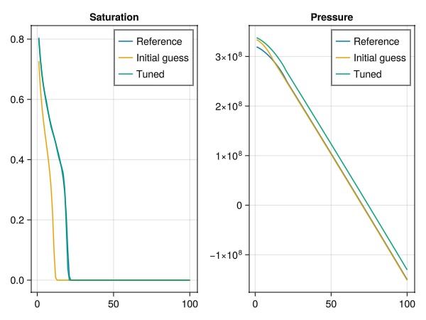

Plot the objective history and function evaluations

fig = Figure()
ax1 = Axis(fig[1, 1], yscale = log10, title = "Objective evaluations", xlabel = "Iterations", ylabel = "Objective")
plot!(ax1, data[:obj_hist][2:end])
ax2 = Axis(fig[1, 2], yscale = log10, title = "Outer optimizer", xlabel = "Iterations", ylabel = "Objective")
t = map(x -> x.value, Optim.trace(results))
plot!(ax2, t)
fig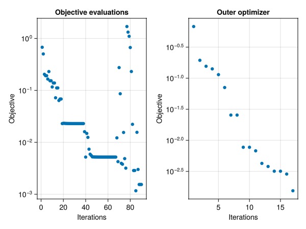

Define an alternative optimization

We can also use the generic interface for optimization, which is a bit less efficient, but a lot more flexible. The previous optimization interface works on numerical parameters (like pore-volumes, transmissibilities, etc.), while the generic interface allows for both numerical and input parameters (like permeability, porosity, etc.).

Note that the viscosity is not defaulted - so we need to let the solver know that it needs to treat it as a distinct parameter, even if we do not optimize on it directly.

opt = setup_reservoir_dict_optimization(case_dporo, parameters = [:PhaseViscosities])
free_optimization_parameter!(opt, [:model, :porosity], rel_min = 0.1, rel_max = 10.0)
prm_opt = optimize_reservoir(opt, saturation_mismatch);
opt

DictParameters with 1 active parameters and 1 inactive:
Active optimization parameters
┌────────────────┬───────────────┬───────┬──────┬─────┬─────────────────┬───────
│           Name │ Initial value │ Count │  Min │ Max │ Optimized value │ Chan ⋯
├────────────────┼───────────────┼───────┼──────┼─────┼─────────────────┼───────
│ model.porosity │ 0.2 ± 0.0     │   100 │ 0.02 │ 2.0 │ 0.182 ± 0.0953  │  -9. ⋯
└────────────────┴───────────────┴───────┴──────┴─────┴─────────────────┴───────
                                                                1 column omitted
Inactive optimization parameters
┌─────────────────────────────┬───────────────────────────────────┬───────┬─────
│                        Name │ Initial value                     │ Count │ Mi ⋯
├─────────────────────────────┼───────────────────────────────────┼───────┼─────
│          model.permeability │ 9.87e-14 ± 1.2600000000000001e-29 │   100 │    ⋯
│          model.rock_density │ 2000.0 ± 0.0                      │   100 │    ⋯
│ parameters.PhaseViscosities │ 0.003 ± 0.002                     │   200 │    ⋯
│             state0.Pressure │ 1.0e8 ± 0.0                       │   100 │    ⋯
│          state0.Saturations │ 0.5 ± 0.5                         │   200 │    ⋯
└─────────────────────────────┴───────────────────────────────────┴───────┴─────
                                                               2 columns omitted

Plot the results

case_opt = opt.setup_function(prm_opt)
states_opt, = simulate(case_opt);

fig = Figure(size = (1200, 600))
ax = Axis(fig[1, 1], title = "Saturation")
lines!(ax, states_ref[end][:Saturations][1, :], label = "Reference")
lines!(ax, states[end][:Saturations][1, :], label = "Initial guess")
lines!(ax, states_tuned[end][:Saturations][1, :], label = "Tuned (Optim)")
lines!(ax, states_opt[end][:Saturations][1, :], label = "Tuned (reservoir_dict_optimization)")

axislegend(ax)
ax = Axis(fig[1, 2], title = "Pressure")
lines!(ax, states_ref[end][:Pressure], label = "Reference")
lines!(ax, states[end][:Pressure], label = "Initial guess")
lines!(ax, states_tuned[end][:Pressure], label = "Tuned (Optim)")
lines!(ax, states_opt[end][:Pressure], label = "Tuned (reservoir_dict_optimization)")
axislegend(ax)
fig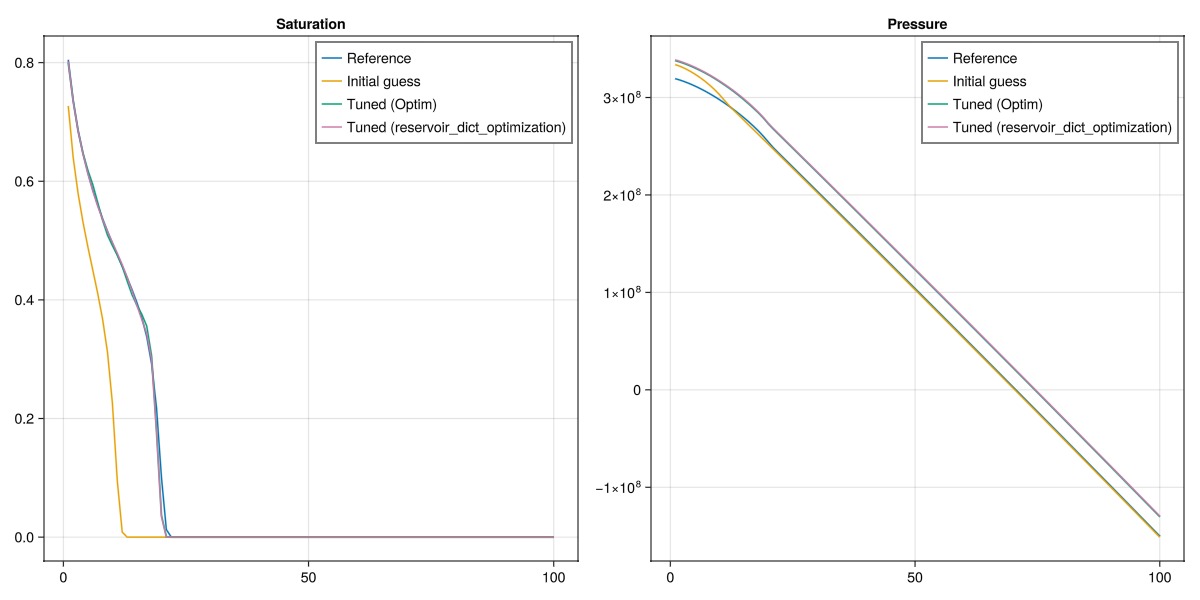

Plot the resulting porosities

Note that the porosity is only changed in the regions where the front has passed. As the objective function measures the difference in saturation, the objective function is only sensitive to the swept region where the saturation has changed.

fig = Figure()
ax = Axis(fig[1, 1], title = "Porosity")
scatter!(ax, prm_opt[:model][:porosity], label = "Optimized porosity")
lines!(ax, states[end][:Saturations][1, :], label = "Final saturation front")
fig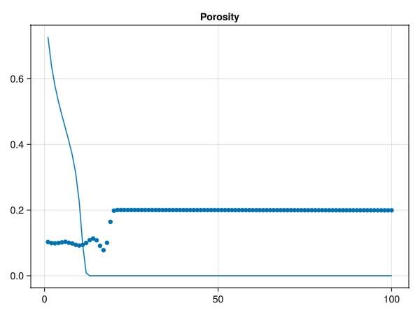

Optimize a single porosity parameter instead

If we introduce the prior assumption that the porosity is constant, we can optimize a single porosity parameter instead of the full porosity field. This is done by writing a setup function that takes a dictionary with the porosity and permeability as input parameters.

function setup_bl(d::AbstractDict, step_info = missing)
    return setup_bl(poro = d[:poro], perm = d[:perm])
end

prm_1poro = Dict(:poro => 0.2, :perm => 0.1*si_unit(:darcy))
opt_1poro = setup_reservoir_dict_optimization(prm_1poro, setup_bl)
free_optimization_parameter!(opt_1poro, :poro, rel_min = 0.1, rel_max = 10.0)
prm_opt_1poro = optimize_reservoir(opt_1poro, saturation_mismatch);
opt_1poro

DictParameters with 1 active parameters and 1 inactive:
Active optimization parameters
┌──────┬───────────────┬───────┬──────┬─────┬─────────────────┬────────┐
│ Name │ Initial value │ Count │  Min │ Max │ Optimized value │ Change │
├──────┼───────────────┼───────┼──────┼─────┼─────────────────┼────────┤
│ poro │ 0.2           │     1 │ 0.02 │ 2.0 │ 0.1             │ -50.0% │
└──────┴───────────────┴───────┴──────┴─────┴─────────────────┴────────┘
Inactive optimization parameters
┌──────┬───────────────┬───────┬─────┬─────┐
│ Name │ Initial value │ Count │ Min │ Max │
├──────┼───────────────┼───────┼─────┼─────┤
│ perm │ 9.87e-14      │     1 │   - │   - │
└──────┴───────────────┴───────┴─────┴─────┘

Plot the results for the single porosity parameter optimization

We observe that we now have recovered the single porosity parameter!

fig = Figure()
ax = Axis(fig[1, 1], title = "Porosity")
scatter!(ax, prm_opt[:model][:porosity], label = "Optimized porosity (all cells)")
scatter!(ax, fill(prm_opt_1poro[:poro], 100), label = "Optimized porosity (single parameter)")
lines!(ax, states[end][:Saturations][1, :], label = "Final saturation front")
axislegend()
fig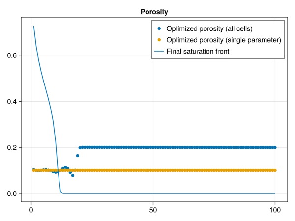

Example on GitHub

If you would like to run this example yourself, it can be downloaded from the JutulDarcy.jl GitHub repository as a script, or as a Jupyter Notebook

This example took 88.78224396 seconds to complete.

---

This page was generated using Literate.jl.