Intro to sensitivities in JutulDarcy

Introduction   Differentiability  

Sensitivites with respect to custom parameters: We demonstrate how to set up a simple conceptual model, add new parameters and variable definitions in the form of a new relative permeability function, and calculate and visualize parameter sensitivities.

We first set up a quarter-five-spot model where the domain is flooded from left to right. Some cells have lower permeability to impede flow and make the scenario more interesting.

For more details, see the paper JutulDarcy.jl - a Fully Differentiable High-Performance Reservoir Simulator Based on Automatic Differentiation.

using Jutul, JutulDarcy, GLMakie
darcy, kg, meter, year, day, bar = si_units(:darcy, :kilogram, :meter, :year, :day, :bar)

L = 1000.0meter
H = 100.0meter
big = false # Paper uses big, takes some more time to run
if big
    nx = 500
else
    nx = 100
end
dx = L/nx

g = reservoir_mesh((nx, nx, 1), (L, L, H))
nc = number_of_cells(g)
perm = fill(0.1darcy, nc)

reservoir = reservoir_domain(g, permeability = 0.1darcy)
centroids = reservoir[:cell_centroids]
rock_type = fill(1, nc)
for (i, x, y) in zip(eachindex(perm), centroids[1, :], centroids[2, :])
    xseg = (x > 0.2L) & (x < 0.8L) & (y > 0.75L) & (y < 0.8L)
    yseg = (y > 0.2L) & (y < 0.8L) & (x > 0.75L) & (x < 0.8L)
    if xseg || yseg
        rock_type[i] = 2
    end
    xseg = (x > 0.2L) & (x < 0.55L) & (y > 0.50L) & (y < 0.55L)
    yseg = (y > 0.2L) & (y < 0.55L) & (x > 0.50L) & (x < 0.55L)
    if xseg || yseg
        rock_type[i] = 3
    end
    xseg = (x > 0.2L) & (x < 0.3L) & (y > 0.25L) & (y < 0.3L)
    yseg = (y > 0.2L) & (y < 0.3L) & (x > 0.25L) & (x < 0.3L)
    if xseg || yseg
        rock_type[i] = 4
    end
end

perm = reservoir[:permeability]
@. perm[rock_type == 2] = 0.001darcy
@. perm[rock_type == 3] = 0.005darcy
@. perm[rock_type == 4] = 0.01darcy

I = setup_vertical_well(reservoir, 1, 1, name = :Injector)
P = setup_vertical_well(reservoir, nx, nx, name = :Producer)

phases = (AqueousPhase(), VaporPhase())
rhoWS, rhoGS = 1000.0kg/meter^3, 700.0kg/meter^3
system = ImmiscibleSystem(phases, reference_densities = (rhoWS, rhoGS))

model = setup_reservoir_model(reservoir, system, wells = [I, P])
rmodel = reservoir_model(model)

SimulationModel:

  Model with 20000 degrees of freedom, 20000 equations and 79600 parameters

  domain:
    DiscretizedDomain with MinimalTPFATopology (10000 cells, 19800 faces) and discretizations for mass_flow, heat_flow

  system:
    ImmiscibleSystem with AqueousPhase, VaporPhase

  context:
    ParallelCSRContext(BlockMajorLayout(false), 1000, 1, MetisPartitioner(:KWAY), :batch)

  formulation:
    FullyImplicitFormulation()

  data_domain:
    DataDomain wrapping UnstructuredMesh with 10000 cells, 19800 faces and 20400 boundary faces with 19 data fields added:
  10000 Cells
    :permeability => 10000 Vector{Float64}
    :porosity => 10000 Vector{Float64}
    :rock_thermal_conductivity => 10000 Vector{Float64}
    :fluid_thermal_conductivity => 10000 Vector{Float64}
    :rock_heat_capacity => 10000 Vector{Float64}
    :component_heat_capacity => 10000 Vector{Float64}
    :rock_density => 10000 Vector{Float64}
    :cell_centroids => 3×10000 Matrix{Float64}
    :volumes => 10000 Vector{Float64}
  19800 Faces
    :neighbors => 2×19800 Matrix{Int64}
    :areas => 19800 Vector{Float64}
    :normals => 3×19800 Matrix{Float64}
    :face_centroids => 3×19800 Matrix{Float64}
  39600 HalfFaces
    :half_face_cells => 39600 Vector{Int64}
    :half_face_faces => 39600 Vector{Int64}
  20400 BoundaryFaces
    :boundary_areas => 20400 Vector{Float64}
    :boundary_centroids => 3×20400 Matrix{Float64}
    :boundary_normals => 3×20400 Matrix{Float64}
    :boundary_neighbors => 20400 Vector{Int64}

  primary_variables:
   1) Pressure    ∈ 10000 Cells: 1 dof each
   2) Saturations ∈ 10000 Cells: 1 dof, 2 values each

  secondary_variables:
   1) PhaseMassDensities     ∈ 10000 Cells: 2 values each
      -> ConstantCompressibilityDensities as evaluator
   2) TotalMasses            ∈ 10000 Cells: 2 values each
      -> TotalMasses as evaluator
   3) RelativePermeabilities ∈ 10000 Cells: 2 values each
      -> BrooksCoreyRelativePermeabilities as evaluator
   4) PhaseMobilities        ∈ 10000 Cells: 2 values each
      -> JutulDarcy.PhaseMobilities as evaluator
   5) PhaseMassMobilities    ∈ 10000 Cells: 2 values each
      -> JutulDarcy.PhaseMassMobilities as evaluator

  parameters:
   1) Transmissibilities        ∈ 19800 Faces: Scalar
   2) TwoPointGravityDifference ∈ 19800 Faces: Scalar
   3) ConnateWater              ∈ 10000 Cells: Scalar
   4) PhaseViscosities          ∈ 10000 Cells: 2 values each
   5) FluidVolume               ∈ 10000 Cells: Scalar

  equations:
   1) mass_conservation ∈ 10000 Cells: 2 values each
      -> ConservationLaw{:TotalMasses, TwoPointPotentialFlowHardCoded{Vector{Int64}, Vector{@NamedTuple{self::Int64, other::Int64, face::Int64, face_sign::Int64}}}, Jutul.DefaultFlux, 2}

  output_variables:
    Pressure, Saturations, TotalMasses

  extra:
    OrderedDict{Symbol, Any} with keys: Symbol[]
  optimization_level:
    1

Plot the initial variable graph

We plot the default variable graph that describes how the different variables relate to each other. When we add a new parameter and property in the next section, the graph is automatically modified.

using NetworkLayout, LayeredLayouts, GraphMakie
Jutul.plot_variable_graph(rmodel)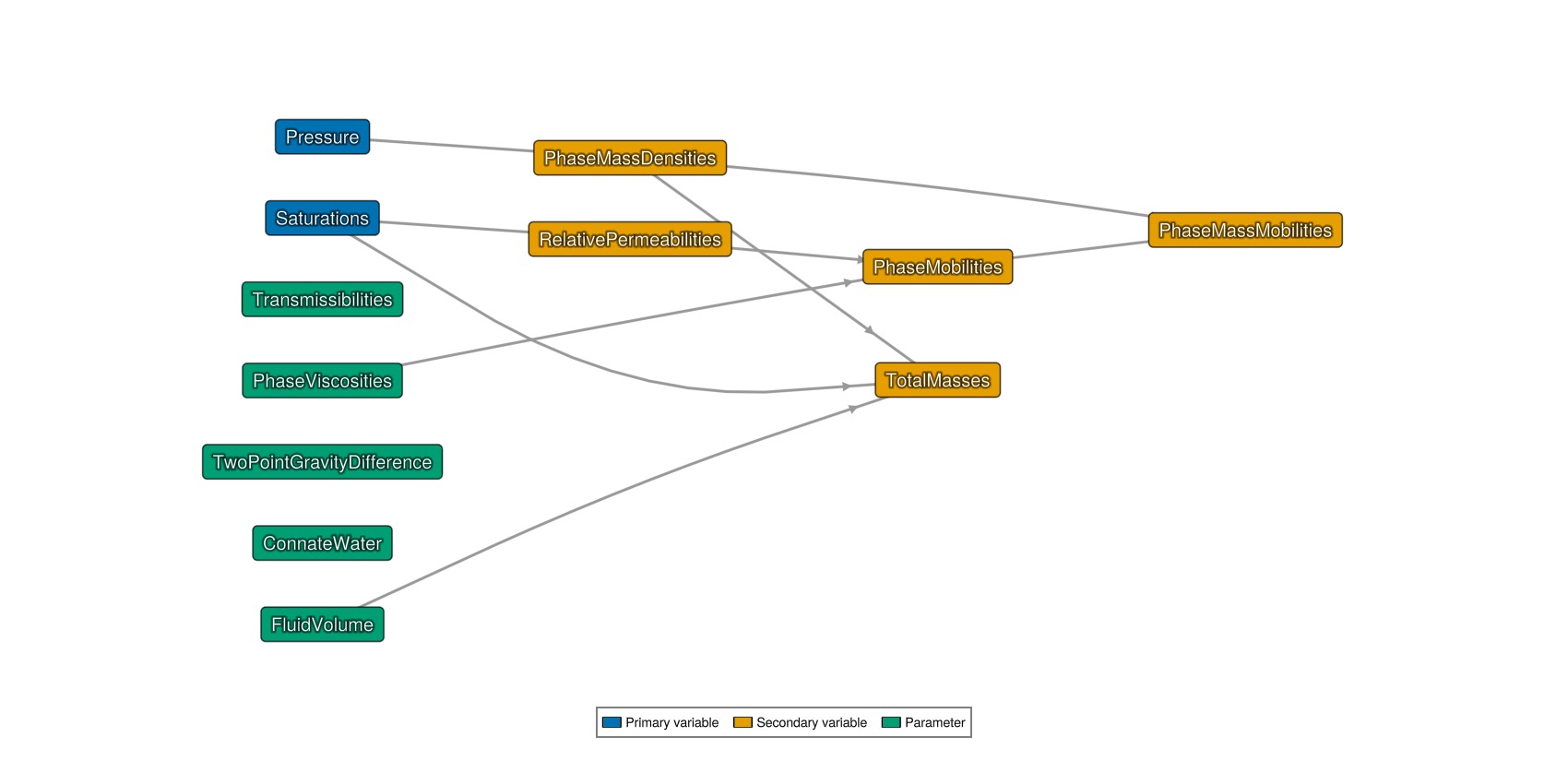

Change the variables

We replace the density variable with a more compressible version, and we also define a new relative permeability variable that depends on a new parameter KrExponents to define the exponent of the relative permeability in each cell and phase of the model.

This is done through several steps:

1. First, we define the type

2. We define functions that act on that type, in particular the update function that is used to evaluate the new relative permeability during the simulation for named inputs Saturations and KrExponents.

3. We define the KrExponents as a model parameter with a default value, that can subsequently be used by the relative permeability.

Finally we plot the variable graph again to verify that the new relationship has been included in our model.

c = [1e-6/bar, 1e-4/bar]
density = ConstantCompressibilityDensities(p_ref = 1*bar, density_ref = [rhoWS, rhoGS], compressibility = c)
replace_variables!(rmodel, PhaseMassDensities = density);

import JutulDarcy: AbstractRelativePermeabilities, PhaseVariables
struct MyKr <: AbstractRelativePermeabilities end
@jutul_secondary function update_my_kr!(vals, def::MyKr, model, Saturations, KrExponents, cells_to_update)
    for c in cells_to_update
        for ph in axes(vals, 1)
            S_α = max(Saturations[ph, c], 0.0)
            n_α = KrExponents[ph, c]
            vals[ph, c] = S_α^n_α
        end
    end
end
struct MyKrExp <: PhaseVariables end
Jutul.default_value(model, ::MyKrExp) = 2.0
set_parameters!(rmodel, KrExponents = MyKrExp())
replace_variables!(rmodel, RelativePermeabilities = MyKr());
Jutul.plot_variable_graph(rmodel)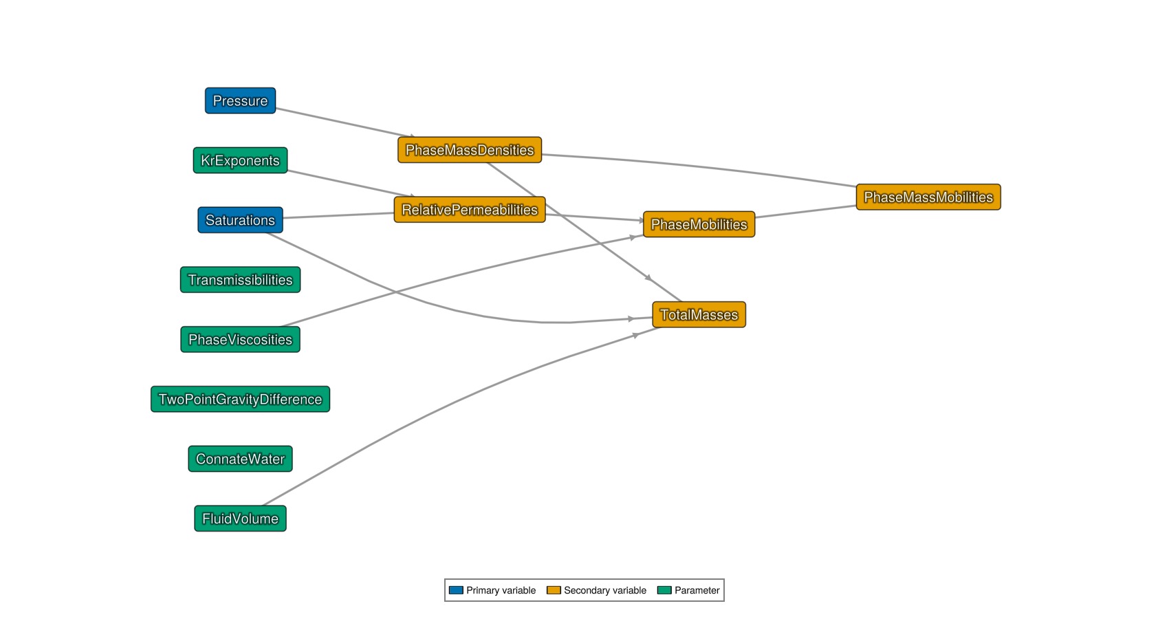

Set up scenario and simulate

parameters = setup_parameters(model)
exponents = parameters[:Reservoir][:KrExponents]
for (cell, rtype) in enumerate(rock_type)
    if rtype == 1
        exp_w = 2
        exp_g = 3
    else
        exp_w = 1
        exp_g = 2
    end
    exponents[1, cell] = exp_w
    exponents[2, cell] = exp_g
end

pv = pore_volume(model, parameters)
state0 = setup_reservoir_state(model, Pressure = 150*bar, Saturations = [1.0, 0.0])

dt = repeat([30.0]*day, 12*5)
pv = pore_volume(model, parameters)
total_time = sum(dt)
inj_rate = sum(pv)/total_time

rate_target = TotalRateTarget(inj_rate)
I_ctrl = InjectorControl(rate_target, [0.0, 1.0], density = rhoGS)
bhp_target = BottomHolePressureTarget(50*bar)
P_ctrl = ProducerControl(bhp_target)
controls = Dict()
controls[:Injector] = I_ctrl
controls[:Producer] = P_ctrl

forces = setup_reservoir_forces(model, control = controls)
case = JutulCase(model, dt, forces, parameters = parameters, state0 = state0)
result = simulate_reservoir(case, output_substates = true);

Jutul: Simulating 4 years, 48.43 weeks as 60 report steps
╭────────────────┬──────────┬───────────────┬──────────╮
│ Iteration type │ Avg/step │  Avg/ministep │    Total │
│                │ 60 steps │ 116 ministeps │ (wasted) │
├────────────────┼──────────┼───────────────┼──────────┤
│ Newton         │  8.81667 │       4.56034 │  529 (0) │
│ Linearization  │    10.75 │       5.56034 │  645 (0) │
│ Linear solver  │  30.3333 │       15.6897 │ 1820 (0) │
│ Precond apply  │  60.6667 │       31.3793 │ 3640 (0) │
╰────────────────┴──────────┴───────────────┴──────────╯
╭───────────────┬─────────┬────────────┬─────────╮
│ Timing type   │    Each │   Relative │   Total │
│               │      ms │ Percentage │       s │
├───────────────┼─────────┼────────────┼─────────┤
│ Properties    │  0.4244 │     0.97 % │  0.2245 │
│ Equations     │ 14.8898 │    41.31 % │  9.6039 │
│ Assembly      │  1.5699 │     4.36 % │  1.0126 │
│ Linear solve  │  1.4537 │     3.31 % │  0.7690 │
│ Linear setup  │  6.9295 │    15.77 % │  3.6657 │
│ Precond apply │  0.6278 │     9.83 % │  2.2851 │
│ Update        │  2.0414 │     4.64 % │  1.0799 │
│ Convergence   │  3.4487 │     9.57 % │  2.2244 │
│ Input/Output  │  0.5119 │     0.26 % │  0.0594 │
│ Other         │  4.3953 │    10.00 % │  2.3251 │
├───────────────┼─────────┼────────────┼─────────┤
│ Total         │ 43.9501 │   100.00 % │ 23.2496 │
╰───────────────┴─────────┴────────────┴─────────╯

Print the gas saturation

ws, states = result
ws(:Producer, :grat)

                             Legend
┌───────┬──────────────────┬──────┬─────────────────────────────┐
│ Label │ Description      │ Unit │ Type of quantity            │
├───────┼──────────────────┼──────┼─────────────────────────────┤
│ grat  │ Surface gas rate │ m³/s │ gas_volume_surface per time │
└───────┴──────────────────┴──────┴─────────────────────────────┘
 Producer result
┌─────────┬──────┐
│    time │ grat │
│    days │ m³/s │
├─────────┼──────┤
│     1.0 │  0.0 │
│ 1.64286 │  0.0 │
│ 2.05612 │  0.0 │
│ 2.98597 │  0.0 │
│ 5.07812 │  0.0 │
│ 8.84401 │  0.0 │
│ 14.4928 │  0.0 │
│ 22.2464 │  0.0 │
│    30.0 │  0.0 │
│ 39.9689 │  0.0 │
│ 49.9844 │  0.0 │
│    60.0 │  0.0 │
│    75.0 │  0.0 │
│    90.0 │  0.0 │
│       ⋮ │    ⋮ │
└─────────┴──────┘
  102 rows omitted

Define objective function

We let the objective function be the amount produced of produced gas, normalized by the injected amount.

using GLMakie
function objective_function(model, state, Δt, step_i, forces)
    grat = JutulDarcy.compute_well_qoi(model, state, forces, :Producer, SurfaceGasRateTarget)
    return Δt*grat/(inj_rate*total_time)
end
data_domain_with_gradients = JutulDarcy.reservoir_sensitivities(case, result, objective_function, include_parameters = true)

DataDomain wrapping UnstructuredMesh with 10000 cells, 19800 faces and 20400 boundary faces with 25 data fields added:
  10000 Cells
    :permeability => 10000 Vector{Float64}
    :porosity => 10000 Vector{Float64}
    :rock_thermal_conductivity => 10000 Vector{Float64}
    :fluid_thermal_conductivity => 10000 Vector{Float64}
    :rock_heat_capacity => 10000 Vector{Float64}
    :component_heat_capacity => 10000 Vector{Float64}
    :rock_density => 10000 Vector{Float64}
    :cell_centroids => 3×10000 Matrix{Float64}
    :volumes => 10000 Vector{Float64}
    :ConnateWater => 10000 Vector{Float64}
    :PhaseViscosities => 2×10000 Matrix{Float64}
    :FluidVolume => 10000 Vector{Float64}
    :KrExponents => 2×10000 Matrix{Float64}
  19800 Faces
    :neighbors => 2×19800 Matrix{Int64}
    :areas => 19800 Vector{Float64}
    :normals => 3×19800 Matrix{Float64}
    :face_centroids => 3×19800 Matrix{Float64}
    :Transmissibilities => 19800 Vector{Float64}
    :TwoPointGravityDifference => 19800 Vector{Float64}
  39600 HalfFaces
    :half_face_cells => 39600 Vector{Int64}
    :half_face_faces => 39600 Vector{Int64}
  20400 BoundaryFaces
    :boundary_areas => 20400 Vector{Float64}
    :boundary_centroids => 3×20400 Matrix{Float64}
    :boundary_normals => 3×20400 Matrix{Float64}
    :boundary_neighbors => 20400 Vector{Int64}

Launch interactive plotter for cell-wise gradients

plot_reservoir(data_domain_with_gradients)

PlotExplorerOutput()

Set up plotting functions

∂K = data_domain_with_gradients[:permeability]
∂ϕ = data_domain_with_gradients[:porosity]

function get_cscale(x)
    minv0, maxv0 = extrema(x)
    minv = min(minv0, -maxv0)
    maxv = max(maxv0, -minv0)
    return (minv, maxv)
end

function myplot(title, vals; kwarg...)
    fig = Figure()
    myplot!(fig, 1, 1, title, vals; kwarg...)
    return fig
end

function myplot!(fig, I, J, title, vals; is_grad = false, is_log = false, colorrange = missing, contourplot = false, nticks = 5, ticks = missing, colorbar = true, kwarg...)
    ax = Axis(fig[I, J], title = title)

    if is_grad
        if ismissing(colorrange)
            colorrange = get_cscale(vals)
        end
        cmap = :seismic
    else
        if ismissing(colorrange)
            colorrange = extrema(vals)
        end
        cmap = :seaborn_icefire_gradient
    end
    hidedecorations!(ax)
    hidespines!(ax)
    arg = (; colormap = cmap, colorrange = colorrange, kwarg...)
    plt = plot_cell_data!(ax, g, vals; shading = NoShading, arg...)
    if colorbar
        if ismissing(ticks)
            ticks = range(colorrange..., nticks)
        end
        Colorbar(fig[I, J+1], plt, ticks = ticks, ticklabelsize = 25, size = 25)
    end
    return fig
end

myplot! (generic function with 1 method)

Plot the permeability

myplot("Permeability", perm./darcy, colorscale = log10, ticks = [0.001, 0.01, 0.1])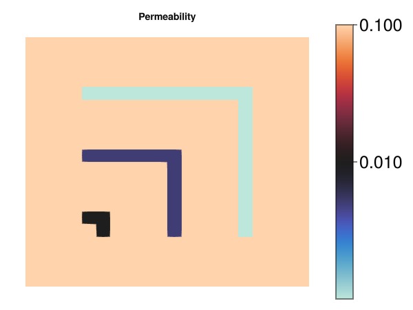

Plot the evolution of the gas saturation

fig = Figure(size = (1200, 400))
sg = states[25][:Saturations][2, :]
myplot!(fig, 1, 1, "Gas saturation", sg, colorrange = (0, 1), colorbar = false)
sg = states[70][:Saturations][2, :]
myplot!(fig, 1, 2, "Gas saturation", sg, colorrange = (0, 1), colorbar = false)
sg = states[end][:Saturations][2, :]
myplot!(fig, 1, 3, "Gas saturation", sg, colorrange = (0, 1))
fig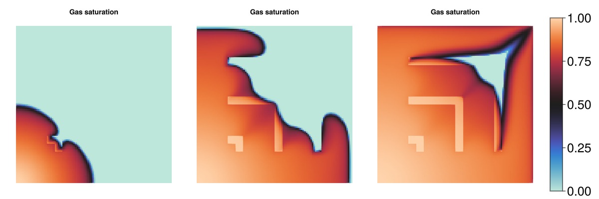

Plot the sensitivity of the objective with respect to permeability

if big
    cr = (-0.001, 0.001)
    cticks = [-0.001, -0.0005, 0.0005, 0.001]
else
    cr = (-0.05, 0.05)
    cticks = [-0.05, -0.025, 0, 0.025, 0.05]
end

myplot("perm_sens", ∂K.*darcy, is_grad = true, ticks = cticks, colorrange = cr)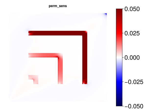

Plot the sensitivity of the objective with respect to porosity

if big
    cr = (-0.00001, 0.00001)
else
    cr = (-0.00025, 0.00025)
end
myplot("porosity_sens", ∂ϕ, is_grad = true, colorrange = cr)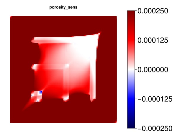

Gradient with respect to cell centroids

∂xyz = data_domain_with_gradients[:cell_centroids]
∂x = ∂xyz[1, :]
∂y = ∂xyz[2, :]
∂z = ∂xyz[3, :]
#
if big
    cr = [-1e-8, 1e-8]
else
    cr = [-1e-7, 1e-7]
end

2-element Vector{Float64}:
 -1.0e-7
  1.0e-7

Plot the sensitivity of the objective with respect to x cell centroids

myplot("dx_sens", ∂x, is_grad = true, colorrange = cr)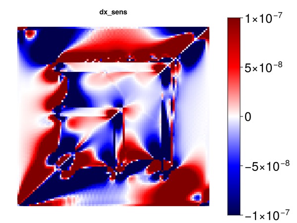

Plot the sensitivity of the objective with respect to y cell centroids

myplot("dy_sens", ∂y, is_grad = true, colorrange = cr)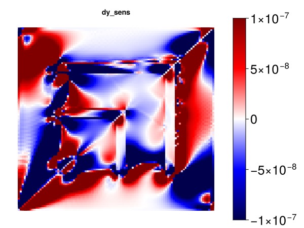

Plot the sensitivity of the objective with respect to z cell centroids

Note: The effect here is primarily coming from gravity.

myplot("dz_sens", ∂z, is_grad = true, colorrange = cr)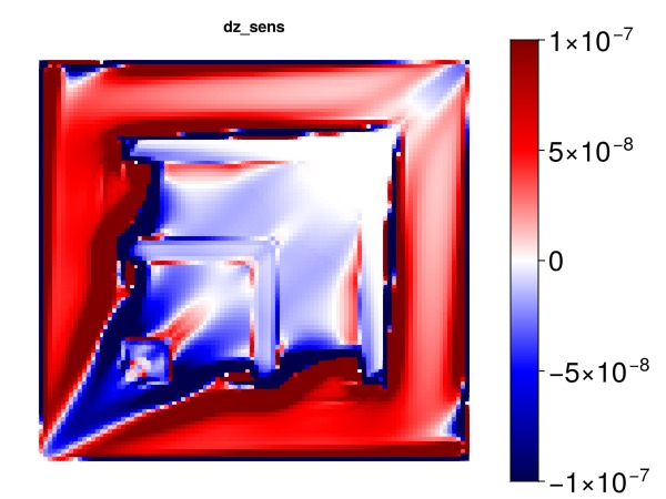

Plot the effect of the new liquid kr exponent on the gas production

if big
    cr = [-1e-7, 1e-7]
else
    cr = [-8e-6, 8e-6]
end

kre = data_domain_with_gradients[:KrExponents]
exp_l = kre[1, :]
myplot("exp_liquid", exp_l, is_grad = true, colorrange = cr)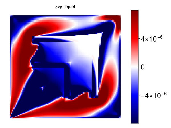

Plot the effect of the new vapor kr exponent on the gas production

exp_v = kre[2, :]
myplot("exp_vapor", exp_v, is_grad = true, colorrange = cr)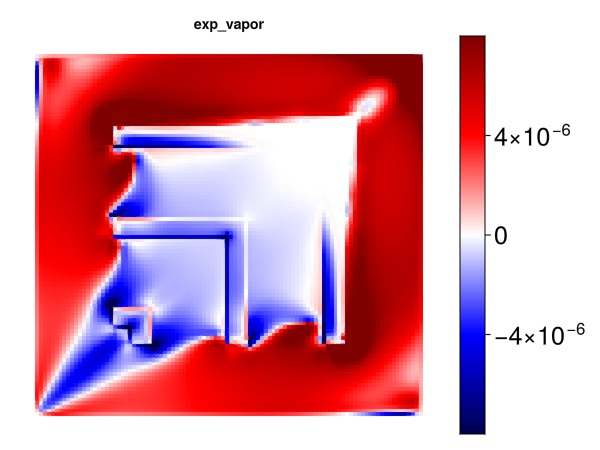

Plot the effect of the liquid phase viscosity

Note: The viscosity can in many models be a variable and not a parameter. For this simple model, however, it is treated as a parameter and we obtain sensitivities.

mu = data_domain_with_gradients[:PhaseViscosities]
if big
    cr = [-0.001, 0.001]
else
    cr = [-0.01, 0.01]
end
mu_l = mu[1, :]
myplot("mu_liquid", mu_l, is_grad = true, colorrange = cr)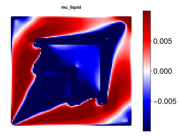

Plot the effect of the liquid phase viscosity

mu_v = mu[2, :]
myplot("mu_vapor", mu_v, is_grad = true, colorrange = cr)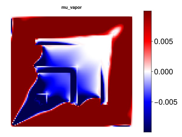

Example on GitHub

If you would like to run this example yourself, it can be downloaded from the JutulDarcy.jl GitHub repository as a script

This example took 159.748049215 seconds to complete.

---

This page was generated using Literate.jl.