Discrete Fracture Model: Validation
Immiscible Geothermal Validation DiscretizationsThis example validates the discrete fracture model (DFM) implementation in JutulDarcy against a full-dimensional reference solution for both a two-phase immiscible and a geothermal system.
Background
Fractures in porous media are thin, high-permeability features that significantly affect fluid flow and heat transport. In this example, we demonstrate two common approaches for modeling fractures:
Full-dimensional (FD): The fracture is explicitly resolved in the mesh as thin cells with high permeability. This is accurate but requires very fine grids to resolve the fracture aperture.
Discrete Fracture Modeling (DFM): The fracture is represented as a codimension-one entity (surface in 3D, line in 2D) embedded in the matrix mesh. Flow between matrix and fracture is handled via cross-terms. This approach avoids the need to resolve the fracture aperture in the mesh and gives much more flexibility in handling complex fracture geometries.
In this example, we set up a fractured cube with an injector–producer doublet and compare the two approaches — first for two-phase immiscible flow and then for geothermal heat transport. We demonstrate that the DFM gives results that closely match the full-dimensional reference in both cases.
Setup
using Jutul, JutulDarcy, GLMakie
import Jutul.CutCellMeshes: PlaneCut, cut_mesh

Darcy, bar, kg, meter, Kelvin, year = si_units(:darcy, :bar, :kilogram, :meter, :Kelvin, :year)
(9.86923266716013e-13, 100000.0, 1.0, 1.0, 1.0, 3.1556952e7)Domain and simulation setup
We create a cube domain with one fracture plane in each coordinate direction, placed at mid-span. The matrix has low permeability, while the fractures have permeability given by the cubic law
The function setup_fractured_cube builds two simulation cases from the same physical domain:
A full-dimensional (FD) Cartesian grid where thin layers of cells explicitly represent the fractures. This serves as the reference solution.
A discrete fracture model (DFM) cut mesh where fractures are embedded surfaces. Cross-terms handle the fracture–matrix coupling.
Both setups share the same injector–producer well pair along the fluid_model keyword (:two_phase or :geothermal) to select the physics and returns ready-to-simulate JutulCase objects.
function setup_fractured_cube(n, L;
        matrix_permeability = 10e-3Darcy,
        matrix_porosity = 0.05,
        fracture_aperture = 1e-4,
        fracture_porosity = 0.5,
        intersection_strategy = :keep,
        well_direction = :z,
        pv_frac = 0.5,
        total_time = year,
        fluid_model = :two_phase,
        temperature = convert_to_si(90.0, :Celsius),
        injection_temperature = convert_to_si(10.0, :Celsius))

    # Normalize input: allow scalar or 3-tuple/vector for n and L.
    dims0 = n isa Integer ? (n, n, n) : Tuple(n)
    Lxyz  = L isa Number  ? (L, L, L) : Tuple(L)
    @assert length(dims0) == 3 "n must be an Int or a length-3 tuple/vector."
    @assert length(Lxyz)  == 3 "L must be a Number or a length-3 tuple/vector."

    # ── Full-dimensional (FD) mesh ──────────────────────────────────────
    # Refine the Cartesian grid around each fracture plane so that a layer of
    # cells with thickness equal to the aperture represents the fracture.
    fd_axis_widths = ntuple(3) do d
        nd = dims0[d]; Ld = Lxyz[d]
        xc = collect(range(0.0, Ld; length = nd + 1))
        xf = Ld / 2
        x = sort(vcat(xc, xf .- fracture_aperture / 2, xf .+ fracture_aperture / 2))
        x = unique(filter(xi -> 0.0 <= xi <= Ld, x))
        diff(x)
    end
    fd_cart_dims = map(length, fd_axis_widths)

    fd_mesh = reservoir_mesh(fd_cart_dims, fd_axis_widths)
    fd_ijk = reinterpret(reshape, Int,
        map(c -> cell_ijk(fd_mesh, c), 1:number_of_cells(fd_mesh)))

    fd_matrix = reservoir_domain(fd_mesh;
        permeability = matrix_permeability, porosity = matrix_porosity)
    is_frac = [any(isapprox.(cell_dims(fd_mesh, c), fracture_aperture; rtol = 1e-2))
               for c in 1:number_of_cells(fd_mesh)]
    fd_matrix[:permeability][is_frac] .= fracture_aperture^2 / 12
    fd_matrix[:porosity][is_frac] .= fracture_porosity
    fd_matrix[:fracture_cells, Cells()] = is_frac

    radius = 0.1
    fd_inj = setup_well(fd_matrix,
        findall(fd_ijk[1, :] .== 1 .&& fd_ijk[2, :] .== 1);
        name = :Injector, simple_well = false, dir = well_direction, radius = radius)
    fd_prod = setup_well(fd_matrix,
        findall(fd_ijk[1, :] .== maximum(fd_ijk[1, :]) .&& fd_ijk[2, :] .== maximum(fd_ijk[2, :]));
        name = :Producer, simple_well = false, dir = well_direction, radius = radius)
    fd_pv = sum(pore_volume(fd_matrix))

    # ── Lower-dimensional (DFM) mesh ────────────────────────────────────
    # Cut a coarse Cartesian grid with fracture planes; the cuts produce an
    # embedded fracture mesh handled by cross-terms.
    ld_mesh = reservoir_mesh(dims0, Lxyz)
    ld_ijk = reinterpret(reshape, Int,
        map(c -> cell_ijk(ld_mesh, c), 1:number_of_cells(ld_mesh)))

    cuts = PlaneCut[]
    for d in 1:3
        center = zeros(3); center[d] = Lxyz[d] / 2
        normal = zeros(3); normal[d] = 1.0
        push!(cuts, PlaneCut(center, normal))
    end

    ld_cut_mesh, info = cut_mesh(ld_mesh, cuts; extra_out = true)
    fracture_faces = findall(info[:face_index] .== 0)
    fracture_mesh = Jutul.EmbeddedMesh(ld_cut_mesh, fracture_faces;
        intersection_strategy = intersection_strategy)
    ld_matrix = reservoir_domain(ld_cut_mesh;
        permeability = matrix_permeability, porosity = matrix_porosity)
    ld_fractures = JutulDarcy.fracture_domain(fracture_mesh, ld_matrix;
        aperture = fracture_aperture, porosity = fracture_porosity)
    ijk = ld_ijk[:, info[:cell_index]]

    # Sort well cells by distance to the corner for consistent ordering.
    function sorted_well_cells(domain, ijk, d1_val, d2_val)
        cells = findall(ijk[1, :] .== d1_val .&& ijk[2, :] .== d2_val)
        x = domain[:cell_centroids][:, cells]
        cells[sortperm(vec(sum(x .^ 2; dims = 1)))]
    end

    inj_cells = sorted_well_cells(ld_matrix, ijk, 1, 1)
    ld_inj = setup_well(ld_matrix, inj_cells;
        name = :Injector, dir = well_direction, radius = radius, simple_well = false)
    prod_cells = sorted_well_cells(ld_matrix, ijk, maximum(ijk[1, :]), maximum(ijk[2, :]))
    ld_prod = setup_well(ld_matrix, prod_cells;
        name = :Producer, dir = well_direction, radius = radius, simple_well = false)

    ld_pv = sum(pore_volume(ld_matrix))
    if ld_fractures !== nothing
        ld_pv += sum(pore_volume(ld_fractures))
    end

    # ── Fluid model selection ───────────────────────────────────────────
    thermal = false

    if fluid_model == :two_phase
        rho = (800.0kg / meter^3, 1000.0kg / meter^3)
        system = ImmiscibleSystem((AqueousPhase(), LiquidPhase());
            reference_densities = rho)
        init = Dict(:Pressure => 50bar, :Saturations => [0.0, 1.0])
        mix = [1.0, 0.0]

    elseif fluid_model == :geothermal
        rho = (1000.0kg / meter^3,)
        system = :geothermal
        init = Dict(:Pressure => 50bar, :Temperature => temperature)
        mix = [1.0]
        thermal = true

    else
        error("Unknown fluid_model = $fluid_model. ",
              "Supported: :two_phase, :geothermal")
    end

    # ── Helper: build a JutulCase from a domain + wells + fractures ─────
    function make_case(matrix, wells, fractures, pv)
        nc = number_of_cells(physical_representation(matrix))

        if isnothing(fractures)
            model = setup_reservoir_model(matrix, system;
                thermal = thermal, wells = wells)
        else
            model = JutulDarcy.setup_fractured_reservoir_model(
                matrix, fractures, system;
                wells = wells, thermal = thermal)
        end

        nstep = 100
        dt = fill(total_time / nstep, nstep)
        rate = pv_frac * pv / sum(dt)

        inj_kwargs = Dict{Symbol, Any}(:density => rho[1])
        if thermal
            inj_kwargs[:temperature] = injection_temperature
        end
        ctrl_inj = InjectorControl(TotalRateTarget(rate), mix; inj_kwargs...)
        ctrl_prod = ProducerControl(BottomHolePressureTarget(10.0bar))

        control = Dict(:Injector => ctrl_inj, :Producer => ctrl_prod)
        forces = setup_reservoir_forces(model; control = control)

        state0 = setup_reservoir_state(model; init...)

        return JutulCase(model, dt, forces; state0 = state0)
    end

    case_fd = make_case(fd_matrix, [fd_inj, fd_prod], nothing, fd_pv)
    case_ld = make_case(ld_matrix, [ld_inj, ld_prod], ld_fractures, ld_pv)

    return (case_fd, case_ld)
end;
Mapping helpers
Map each DFM cell (matrix and fracture) to the nearest FD cell so that we can compute pointwise errors between the two solutions.
function map_dfm_to_fd(fd_domain, dfm_domain, dfm_fractures)
    x_fd = fd_domain[:cell_centroids]
    nearest(x) = last(findmin(vec(sum((x .- x_fd) .^ 2; dims = 1))))
    ld2fd_m = [nearest(c) for c in eachcol(dfm_domain[:cell_centroids])]
    ld2fd_f = [nearest(c) for c in eachcol(dfm_fractures[:cell_centroids])]
    return ld2fd_m, ld2fd_f
end

function reconstruct_full_state(state_m, state_f, state_fd, ld2fd_m, ld2fd_f)
    full = deepcopy(state_fd)
    nc = length(state_m[:Pressure])
    for k in keys(state_m)
        v, vm, vf = full[k], state_m[k], state_f[k]
        if vm isa Vector && length(vm) == nc
            v[ld2fd_m] .= vm
            v[ld2fd_f] .= vf
        elseif vm isa AbstractArray && size(vm, 2) == nc
            v[:, ld2fd_m] .= vm
            v[:, ld2fd_f] .= vf
        end
        full[k] = v
    end
    return full
end;
Part 1 – Two-phase immiscible validation
We first validate the DFM for a two-phase immiscible system. A liquid phase displaces the aqueous phase through the fractured cube. The injection rate is chosen so that 5 pore volumes are injected in one year.
cart_dims = (21, 21, 5)
phys_dims = (100.0, 100.0, 10.0)

case_fd_tp, case_dfm_tp = setup_fractured_cube(
    cart_dims, phys_dims;
    fluid_model = :two_phase,
    matrix_permeability = 1e-2Darcy,
    matrix_porosity = 0.01,
    fracture_aperture = 1e-4,
    pv_frac = 5.0,
    total_time = year);
Simulate both cases.
sim_args = (info_level = 0, max_nonlinear_iterations = 15, max_timestep_cuts = 25)
res_fd_tp = simulate_reservoir(case_fd_tp; sim_args...)
res_dfm_tp = simulate_reservoir(case_dfm_tp; sim_args...);
Jutul: Simulating 1 year as 100 report steps
╭────────────────┬───────────┬───────────────┬───────────╮
│ Iteration type │ Avg/step │ Avg/ministep │ Total │
│ │ 100 steps │ 107 ministeps │ (wasted) │
├────────────────┼───────────┼───────────────┼───────────┤
│ Newton │ 3.64 │ 3.40187 │ 364 (15) │
│ Linearization │ 4.71 │ 4.40187 │ 471 (16) │
│ Linear solver │ 4.55 │ 4.25234 │ 455 (62) │
│ Precond apply │ 9.1 │ 8.50467 │ 910 (124) │
╰────────────────┴───────────┴───────────────┴───────────╯
╭───────────────┬─────────┬────────────┬─────────╮
│ Timing type │ Each │ Relative │ Total │
│ │ ms │ Percentage │ s │
├───────────────┼─────────┼────────────┼─────────┤
│ Properties │ 0.3623 │ 1.00 % │ 0.1319 │
│ Equations │ 9.7826 │ 34.93 % │ 4.6076 │
│ Assembly │ 5.1900 │ 18.53 % │ 2.4445 │
│ Linear solve │ 0.6459 │ 1.78 % │ 0.2351 │
│ Linear setup │ 3.4513 │ 9.52 % │ 1.2563 │
│ Precond apply │ 0.3191 │ 2.20 % │ 0.2904 │
│ Update │ 1.5205 │ 4.20 % │ 0.5535 │
│ Convergence │ 3.7162 │ 13.27 % │ 1.7503 │
│ Input/Output │ 0.7322 │ 0.59 % │ 0.0783 │
│ Other │ 5.0618 │ 13.97 % │ 1.8425 │
├───────────────┼─────────┼────────────┼─────────┤
│ Total │ 36.2373 │ 100.00 % │ 13.1904 │
╰───────────────┴─────────┴────────────┴─────────╯
Jutul: Simulating 1 year as 100 report steps
╭────────────────┬───────────┬───────────────┬──────────╮
│ Iteration type │ Avg/step │ Avg/ministep │ Total │
│ │ 100 steps │ 105 ministeps │ (wasted) │
├────────────────┼───────────┼───────────────┼──────────┤
│ Newton │ 3.15 │ 3.0 │ 315 (0) │
│ Linearization │ 4.2 │ 4.0 │ 420 (0) │
│ Linear solver │ 3.7 │ 3.52381 │ 370 (0) │
│ Precond apply │ 7.4 │ 7.04762 │ 740 (0) │
╰────────────────┴───────────┴───────────────┴──────────╯
╭───────────────┬─────────┬────────────┬─────────╮
│ Timing type │ Each │ Relative │ Total │
│ │ ms │ Percentage │ s │
├───────────────┼─────────┼────────────┼─────────┤
│ Properties │ 0.3945 │ 0.89 % │ 0.1243 │
│ Equations │ 13.5067 │ 40.44 % │ 5.6728 │
│ Assembly │ 4.0404 │ 12.10 % │ 1.6970 │
│ Linear solve │ 1.6727 │ 3.76 % │ 0.5269 │
│ Linear setup │ 5.1300 │ 11.52 % │ 1.6159 │
│ Precond apply │ 0.3055 │ 1.61 % │ 0.2260 │
│ Update │ 1.7795 │ 4.00 % │ 0.5606 │
│ Convergence │ 3.4976 │ 10.47 % │ 1.4690 │
│ Input/Output │ 1.0368 │ 0.78 % │ 0.1089 │
│ Other │ 6.4281 │ 14.44 % │ 2.0248 │
├───────────────┼─────────┼────────────┼─────────┤
│ Total │ 44.5275 │ 100.00 % │ 14.0262 │
╰───────────────┴─────────┴────────────┴─────────╯Two-phase well comparison
If the DFM correctly reproduces the fracture physics, injection and production curves should closely follow the full-dimensional reference.
plot_well_results([res_fd_tp.wells, res_dfm_tp.wells];
    names = ["Full-dimensional", "DFM"])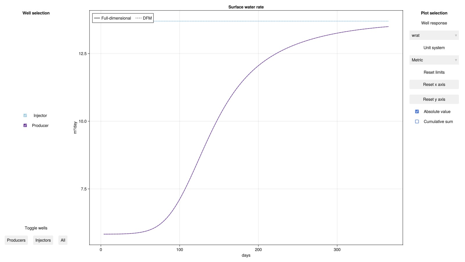
Two-phase cell-wise error
Map the DFM solution back onto the FD grid and compute cell-wise saturation differences.
fd_domain_tp = case_fd_tp.model[:Reservoir].data_domain
dfm_domain_tp = case_dfm_tp.model[:Reservoir].data_domain
dfm_fractures_tp = case_dfm_tp.model[:Fractures].data_domain
ld2fd_m_tp, ld2fd_f_tp = map_dfm_to_fd(fd_domain_tp, dfm_domain_tp, dfm_fractures_tp)

states_fd_tp = map(s -> s[:Reservoir], res_fd_tp.result.states)
states_dfm_tp = map(s -> s[:Reservoir], res_dfm_tp.result.states)
states_frac_tp = map(s -> s[:Fractures], res_dfm_tp.result.states)

states_recon_tp = [
    reconstruct_full_state(sm, sf, sfd, ld2fd_m_tp, ld2fd_f_tp)
    for (sm, sf, sfd) in zip(states_dfm_tp, states_frac_tp, states_fd_tp)
]
delta_tp = JutulDarcy.delta_state(states_recon_tp, states_fd_tp)
plot_reservoir(case_fd_tp.model[:Reservoir], delta_tp; key = :Saturations)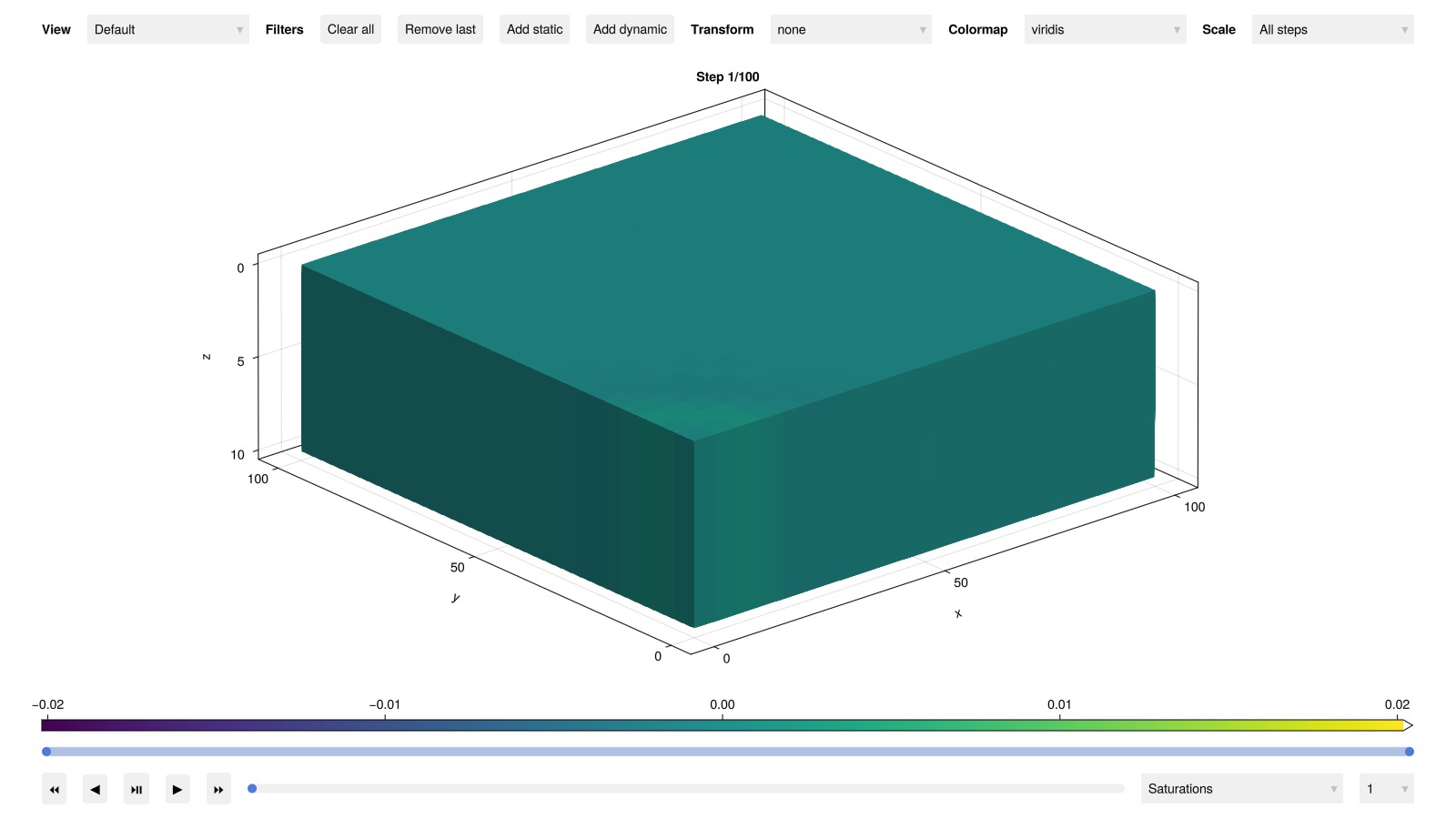
Part 2 – Geothermal validation
Next we validate the DFM for a single-phase geothermal system. Cold water (10 °C) is injected into a hot reservoir (90 °C), with fractures acting as preferential pathways for heat transport. We inject 50 pore volumes over one year so that the cold water has time to cool down the surrounding rock.
case_fd_gt, case_dfm_gt = setup_fractured_cube(
    cart_dims, phys_dims;
    fluid_model = :geothermal,
    matrix_permeability = 1e-3Darcy,
    matrix_porosity = 0.01,
    fracture_aperture = 1e-4,
    pv_frac = 50.0,
    total_time = year,
    temperature = convert_to_si(90.0, :Celsius),
    injection_temperature = convert_to_si(10.0, :Celsius));
Simulate both cases.
sim_args_gt = (info_level = 0, initial_dt = 5.0)
res_fd_gt = simulate_reservoir(case_fd_gt; sim_args_gt...)
res_dfm_gt = simulate_reservoir(case_dfm_gt; sim_args_gt...);
Jutul: Simulating 1 year as 100 report steps
╭────────────────┬───────────┬───────────────┬──────────╮
│ Iteration type │ Avg/step │ Avg/ministep │ Total │
│ │ 100 steps │ 202 ministeps │ (wasted) │
├────────────────┼───────────┼───────────────┼──────────┤
│ Newton │ 8.52 │ 4.21782 │ 852 (0) │
│ Linearization │ 10.54 │ 5.21782 │ 1054 (0) │
│ Linear solver │ 32.12 │ 15.901 │ 3212 (0) │
│ Precond apply │ 64.24 │ 31.802 │ 6424 (0) │
╰────────────────┴───────────┴───────────────┴──────────╯
╭───────────────┬─────────┬────────────┬─────────╮
│ Timing type │ Each │ Relative │ Total │
│ │ ms │ Percentage │ s │
├───────────────┼─────────┼────────────┼─────────┤
│ Properties │ 0.4520 │ 1.36 % │ 0.3851 │
│ Equations │ 10.8161 │ 40.13 % │ 11.4002 │
│ Assembly │ 2.9178 │ 10.83 % │ 3.0754 │
│ Linear solve │ 0.6915 │ 2.07 % │ 0.5892 │
│ Linear setup │ 3.9331 │ 11.80 % │ 3.3510 │
│ Precond apply │ 0.2948 │ 6.67 % │ 1.8935 │
│ Update │ 2.5114 │ 7.53 % │ 2.1397 │
│ Convergence │ 2.7928 │ 10.36 % │ 2.9436 │
│ Input/Output │ 0.8534 │ 0.61 % │ 0.1724 │
│ Other │ 2.8832 │ 8.65 % │ 2.4565 │
├───────────────┼─────────┼────────────┼─────────┤
│ Total │ 33.3410 │ 100.00 % │ 28.4065 │
╰───────────────┴─────────┴────────────┴─────────╯
Jutul: Simulating 1 year as 100 report steps
╭────────────────┬───────────┬───────────────┬──────────╮
│ Iteration type │ Avg/step │ Avg/ministep │ Total │
│ │ 100 steps │ 219 ministeps │ (wasted) │
├────────────────┼───────────┼───────────────┼──────────┤
│ Newton │ 9.56 │ 4.3653 │ 956 (0) │
│ Linearization │ 11.75 │ 5.3653 │ 1175 (0) │
│ Linear solver │ 36.86 │ 16.8311 │ 3686 (0) │
│ Precond apply │ 73.72 │ 33.6621 │ 7372 (0) │
╰────────────────┴───────────┴───────────────┴──────────╯
╭───────────────┬─────────┬────────────┬─────────╮
│ Timing type │ Each │ Relative │ Total │
│ │ ms │ Percentage │ s │
├───────────────┼─────────┼────────────┼─────────┤
│ Properties │ 0.5644 │ 2.09 % │ 0.5395 │
│ Equations │ 10.6202 │ 48.33 % │ 12.4788 │
│ Assembly │ 1.4585 │ 6.64 % │ 1.7137 │
│ Linear solve │ 0.6908 │ 2.56 % │ 0.6604 │
│ Linear setup │ 3.5892 │ 13.29 % │ 3.4313 │
│ Precond apply │ 0.2712 │ 7.74 % │ 1.9994 │
│ Update │ 0.7367 │ 2.73 % │ 0.7043 │
│ Convergence │ 1.8060 │ 8.22 % │ 2.1220 │
│ Input/Output │ 0.5285 │ 0.45 % │ 0.1158 │
│ Other │ 2.1480 │ 7.95 % │ 2.0535 │
├───────────────┼─────────┼────────────┼─────────┤
│ Total │ 27.0069 │ 100.00 % │ 25.8186 │
╰───────────────┴─────────┴────────────┴─────────╯Geothermal well comparison
The key metric is the thermal breakthrough time: when the cold injected water reaches the producer. If the DFM correctly captures the fracture flow paths, the production temperature should closely track the full-dimensional reference.
plot_well_results([res_fd_gt.wells, res_dfm_gt.wells],
    names = ["Full-dimensional", "DFM"])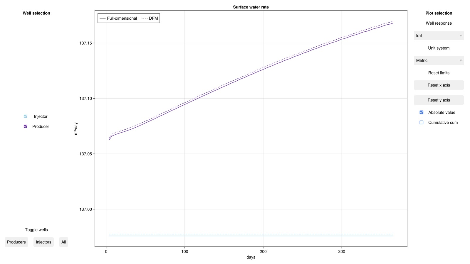
Geothermal cell-wise temperature error
Map the DFM solution onto the FD grid and plot the cell-wise temperature difference. Small differences confirm that the DFM faithfully captures thermal transport through fractures.
fd_domain_gt = case_fd_gt.model[:Reservoir].data_domain
dfm_domain_gt = case_dfm_gt.model[:Reservoir].data_domain
dfm_fractures_gt = case_dfm_gt.model[:Fractures].data_domain
ld2fd_m_gt, ld2fd_f_gt = map_dfm_to_fd(fd_domain_gt, dfm_domain_gt, dfm_fractures_gt)

states_fd_gt = map(s -> s[:Reservoir], res_fd_gt.result.states)
states_dfm_gt = map(s -> s[:Reservoir], res_dfm_gt.result.states)
states_frac_gt = map(s -> s[:Fractures], res_dfm_gt.result.states)

states_recon_gt = [
    reconstruct_full_state(sm, sf, sfd, ld2fd_m_gt, ld2fd_f_gt)
    for (sm, sf, sfd) in zip(states_dfm_gt, states_frac_gt, states_fd_gt)
]
delta_gt = JutulDarcy.delta_state(states_recon_gt, states_fd_gt)
plot_reservoir(case_fd_gt.model[:Reservoir], delta_gt; key = :Temperature)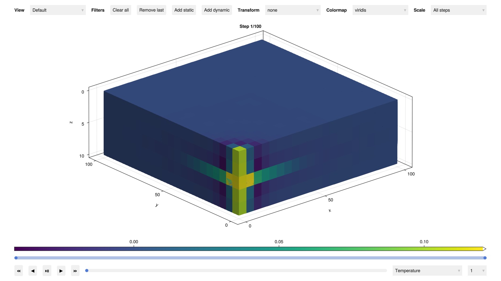
Example on GitHub
If you would like to run this example yourself, it can be downloaded from the JutulDarcy.jl GitHub repository as a script
This example took 239.040630879 seconds to complete.This page was generated using Literate.jl.