SPE10, model 2

Introduction   InputFile  

The SPE10 benchmark case is a standard benchmark case for reservoir simulators. The model is described in detail in the SPE10 benchmark page

This example demonstrates routines to set up the SPE10, model 2, case using premade functions in the JutulDarcy.SPE10 module. This model is often just called SPE10, since the first model of the benchmark is very small.

Set up the reservoir

We can set up the reservoir itself to have a look at the static properties.

using JutulDarcy, GLMakie, HYPRE
reservoir = JutulDarcy.SPE10.setup_reservoir()
plot_reservoir(reservoir, key = :porosity)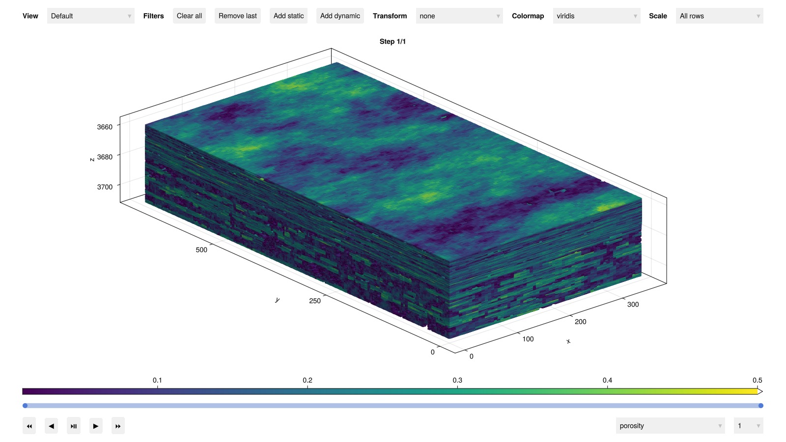

Set up and run a simulation for the first layer

We can set up and run a full simulation for the first layer of the model. As we want the example to run quickly, we just pick the top layer. The function is set up to scale the default well rates to the smaller model, so you can adjust the number of layers without changing anything else.

case = JutulDarcy.SPE10.setup_case(layers = 1:1)

Jutul case with 100 time-steps (5 years, 24 weeks, 5.787 days) and constant forces for all steps.

Model:

MultiModel with 7 models and 20 cross-terms. 26238 equations, 26238 degrees of freedom and 77841 parameters.

  models:
    1) Reservoir (26208x26208)
       ImmiscibleSystem with AqueousPhase, LiquidPhase
       ∈ MinimalTPFATopology (13104 cells, 25809 faces)
    2) I1 (2x2)
       ImmiscibleSystem with AqueousPhase, LiquidPhase
       ∈ SimpleWell [I1] (1 nodes, 0 segments, 1 perforations)
    3) P1 (2x2)
       ImmiscibleSystem with AqueousPhase, LiquidPhase
       ∈ SimpleWell [P1] (1 nodes, 0 segments, 1 perforations)
    4) P2 (2x2)
       ImmiscibleSystem with AqueousPhase, LiquidPhase
       ∈ SimpleWell [P2] (1 nodes, 0 segments, 1 perforations)
    5) P3 (2x2)
       ImmiscibleSystem with AqueousPhase, LiquidPhase
       ∈ SimpleWell [P3] (1 nodes, 0 segments, 1 perforations)
    6) P4 (2x2)
       ImmiscibleSystem with AqueousPhase, LiquidPhase
       ∈ SimpleWell [P4] (1 nodes, 0 segments, 1 perforations)
    7) Facility (20x20)
       JutulDarcy.FacilitySystem{ImmiscibleSystem{Tuple{AqueousPhase, LiquidPhase}, Tuple{Float64, Float64}}}(ImmiscibleSystem with AqueousPhase, LiquidPhase)
       ∈ WellGroup([:I1, :P1, :P2, :P3, :P4], true, true)

  cross_terms:
    1) I1 <-> Reservoir (Eqs: mass_conservation <-> mass_conservation)
       JutulDarcy.ReservoirFromWellFlowCT
    2) P1 <-> Reservoir (Eqs: mass_conservation <-> mass_conservation)
       JutulDarcy.ReservoirFromWellFlowCT
    3) P2 <-> Reservoir (Eqs: mass_conservation <-> mass_conservation)
       JutulDarcy.ReservoirFromWellFlowCT
    4) P3 <-> Reservoir (Eqs: mass_conservation <-> mass_conservation)
       JutulDarcy.ReservoirFromWellFlowCT
    5) P4 <-> Reservoir (Eqs: mass_conservation <-> mass_conservation)
       JutulDarcy.ReservoirFromWellFlowCT
    6) Facility  -> I1 (Eq: mass_conservation)
       JutulDarcy.WellFromFacilityFlowCT
    7) I1  -> Facility (Eq: bottom_hole_pressure_equation)
       JutulDarcy.FacilityFromWellBottomHolePressureCT
    8) I1  -> Facility (Eq: surface_phase_rates_equation)
       JutulDarcy.FacilityFromSurfacePhaseRatesCT
    9) Facility  -> P1 (Eq: mass_conservation)
       JutulDarcy.WellFromFacilityFlowCT
    10) P1  -> Facility (Eq: bottom_hole_pressure_equation)
       JutulDarcy.FacilityFromWellBottomHolePressureCT
    11) P1  -> Facility (Eq: surface_phase_rates_equation)
       JutulDarcy.FacilityFromSurfacePhaseRatesCT
    12) Facility  -> P2 (Eq: mass_conservation)
       JutulDarcy.WellFromFacilityFlowCT
    13) P2  -> Facility (Eq: bottom_hole_pressure_equation)
       JutulDarcy.FacilityFromWellBottomHolePressureCT
    14) P2  -> Facility (Eq: surface_phase_rates_equation)
       JutulDarcy.FacilityFromSurfacePhaseRatesCT
    15) Facility  -> P3 (Eq: mass_conservation)
       JutulDarcy.WellFromFacilityFlowCT
    16) P3  -> Facility (Eq: bottom_hole_pressure_equation)
       JutulDarcy.FacilityFromWellBottomHolePressureCT
    17) P3  -> Facility (Eq: surface_phase_rates_equation)
       JutulDarcy.FacilityFromSurfacePhaseRatesCT
    18) Facility  -> P4 (Eq: mass_conservation)
       JutulDarcy.WellFromFacilityFlowCT
    19) P4  -> Facility (Eq: bottom_hole_pressure_equation)
       JutulDarcy.FacilityFromWellBottomHolePressureCT
    20) P4  -> Facility (Eq: surface_phase_rates_equation)
       JutulDarcy.FacilityFromSurfacePhaseRatesCT

Model storage will be optimized for runtime performance.

Plot the porosity

Note that some cells are removed due to very low porosity. The setup function has additional options to control this behavior if you would rather limit the minimum porosity than removing cells.

plot_reservoir(case.model, key = :porosity)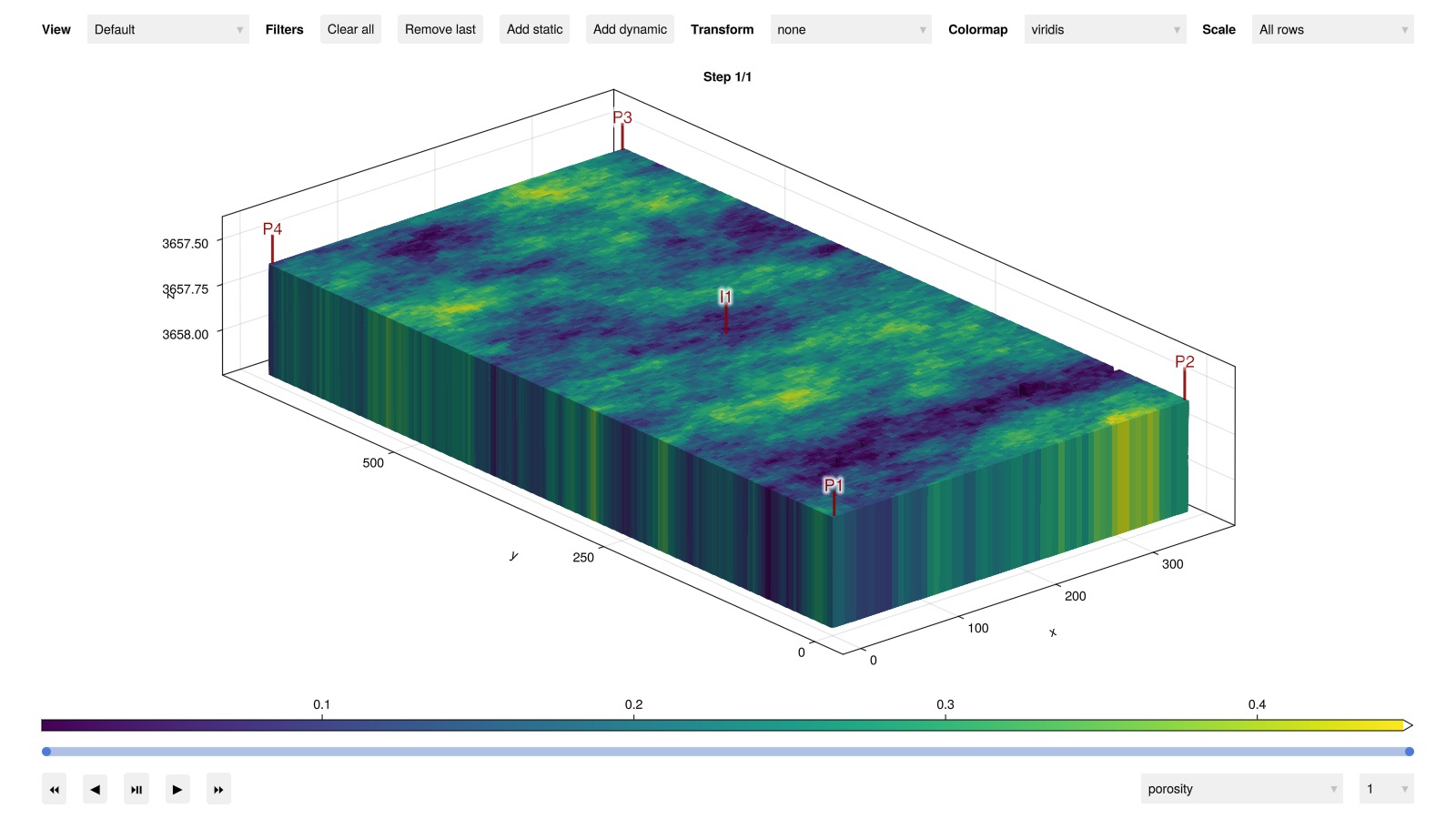

Run the simulation

ws, states = simulate_reservoir(case)

ReservoirSimResult with 100 entries:

  wells (5 present):
    :P1
    :P3
    :P4
    :I1
    :P2
    Results per well:
       :wrat => Vector{Float64} of size (100,)
       :Aqueous_mass_rate => Vector{Float64} of size (100,)
       :orat => Vector{Float64} of size (100,)
       :bhp => Vector{Float64} of size (100,)
       :mrat => Vector{Float64} of size (100,)
       :lrat => Vector{Float64} of size (100,)
       :mass_rate => Vector{Float64} of size (100,)
       :rate => Vector{Float64} of size (100,)
       :control => Vector{Symbol} of size (100,)
       :Liquid_mass_rate => Vector{Float64} of size (100,)
       :wcut => Vector{Float64} of size (100,)

  states (Vector with 100 entries, reservoir variables for each state)
    :Pressure => Vector{Float64} of size (13104,)
    :Saturations => Matrix{Float64} of size (2, 13104)
    :TotalMasses => Matrix{Float64} of size (2, 13104)

  time (report time for each state)
     Vector{Float64} of length 100

  result (extended states, reports)
     SimResult with 100 entries

  extra
     Dict{Any, Any} with keys :simulator, :config

  Completed at Dec. 19 2025 12:48 after 15 seconds, 794 milliseconds, 696.8 microseconds.

Plot the final saturation

plot_reservoir(case.model, states, key = :Saturations, step = length(states))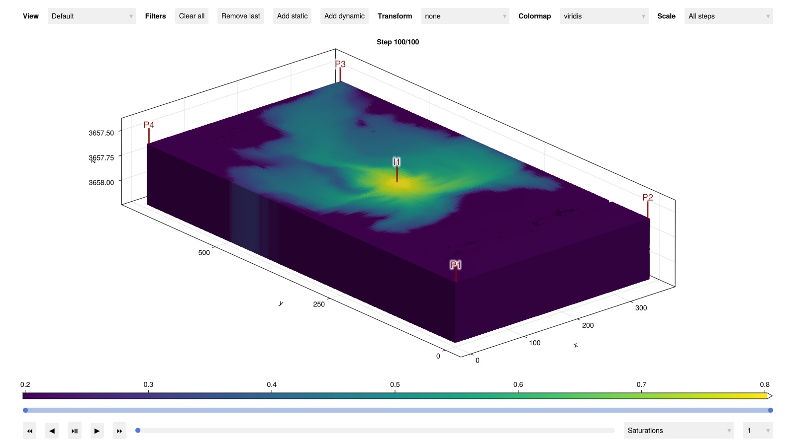

Show the last layer

The first 35 layers correspond to the Tarbert formation and the latter 50 layers are the upper ness formation. We plot one of the last layers, showing a channelized, fluvial structure.

reservoir_ness = JutulDarcy.SPE10.setup_reservoir(layers = 60)
plot_reservoir(reservoir_ness, key = :porosity)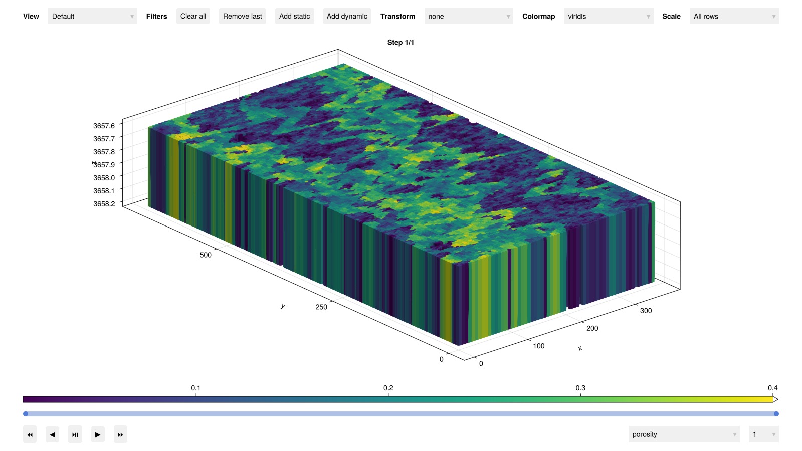

Coarsen the model

The full model is quite large, with 1.1 million cells. We can coarsen the model to get a smaller model that is faster to simulate. The original model was intended as a benchmark for upscaling methods, even though such models are now quite easy to simulate when using parallel computing on CPU/GPU.

The default coarsening is quite simple (harmonic averages and sums), but quickly sets up a coarse model that can be used for testing, or as a starting point for a more refined coarsening.

case_fine = JutulDarcy.SPE10.setup_case()
case_coarse = coarsen_reservoir_case(case_fine, (10, 22, 40))

Jutul case with 100 time-steps (5 years, 24 weeks, 5.787 days) and constant forces for all steps.

Model:

MultiModel with 7 models and 20 cross-terms. 18598 equations, 18598 degrees of freedom and 72217 parameters.

  models:
    1) Reservoir (18568x18568)
       ImmiscibleSystem with AqueousPhase, LiquidPhase
       ∈ MinimalTPFATopology (9284 cells, 26624 faces)
    2) I1 (2x2)
       ImmiscibleSystem with AqueousPhase, LiquidPhase
       ∈ SimpleWell [I1] (1 nodes, 0 segments, 40 perforations)
    3) P1 (2x2)
       ImmiscibleSystem with AqueousPhase, LiquidPhase
       ∈ SimpleWell [P1] (1 nodes, 0 segments, 39 perforations)
    4) P2 (2x2)
       ImmiscibleSystem with AqueousPhase, LiquidPhase
       ∈ SimpleWell [P2] (1 nodes, 0 segments, 39 perforations)
    5) P3 (2x2)
       ImmiscibleSystem with AqueousPhase, LiquidPhase
       ∈ SimpleWell [P3] (1 nodes, 0 segments, 40 perforations)
    6) P4 (2x2)
       ImmiscibleSystem with AqueousPhase, LiquidPhase
       ∈ SimpleWell [P4] (1 nodes, 0 segments, 40 perforations)
    7) Facility (20x20)
       JutulDarcy.FacilitySystem{ImmiscibleSystem{Tuple{AqueousPhase, LiquidPhase}, Tuple{Float64, Float64}}}(ImmiscibleSystem with AqueousPhase, LiquidPhase)
       ∈ WellGroup([:I1, :P1, :P2, :P3, :P4], true, true)

  cross_terms:
    1) I1 <-> Reservoir (Eqs: mass_conservation <-> mass_conservation)
       JutulDarcy.ReservoirFromWellFlowCT
    2) P1 <-> Reservoir (Eqs: mass_conservation <-> mass_conservation)
       JutulDarcy.ReservoirFromWellFlowCT
    3) P2 <-> Reservoir (Eqs: mass_conservation <-> mass_conservation)
       JutulDarcy.ReservoirFromWellFlowCT
    4) P3 <-> Reservoir (Eqs: mass_conservation <-> mass_conservation)
       JutulDarcy.ReservoirFromWellFlowCT
    5) P4 <-> Reservoir (Eqs: mass_conservation <-> mass_conservation)
       JutulDarcy.ReservoirFromWellFlowCT
    6) Facility  -> I1 (Eq: mass_conservation)
       JutulDarcy.WellFromFacilityFlowCT
    7) I1  -> Facility (Eq: bottom_hole_pressure_equation)
       JutulDarcy.FacilityFromWellBottomHolePressureCT
    8) I1  -> Facility (Eq: surface_phase_rates_equation)
       JutulDarcy.FacilityFromSurfacePhaseRatesCT
    9) Facility  -> P1 (Eq: mass_conservation)
       JutulDarcy.WellFromFacilityFlowCT
    10) P1  -> Facility (Eq: bottom_hole_pressure_equation)
       JutulDarcy.FacilityFromWellBottomHolePressureCT
    11) P1  -> Facility (Eq: surface_phase_rates_equation)
       JutulDarcy.FacilityFromSurfacePhaseRatesCT
    12) Facility  -> P2 (Eq: mass_conservation)
       JutulDarcy.WellFromFacilityFlowCT
    13) P2  -> Facility (Eq: bottom_hole_pressure_equation)
       JutulDarcy.FacilityFromWellBottomHolePressureCT
    14) P2  -> Facility (Eq: surface_phase_rates_equation)
       JutulDarcy.FacilityFromSurfacePhaseRatesCT
    15) Facility  -> P3 (Eq: mass_conservation)
       JutulDarcy.WellFromFacilityFlowCT
    16) P3  -> Facility (Eq: bottom_hole_pressure_equation)
       JutulDarcy.FacilityFromWellBottomHolePressureCT
    17) P3  -> Facility (Eq: surface_phase_rates_equation)
       JutulDarcy.FacilityFromSurfacePhaseRatesCT
    18) Facility  -> P4 (Eq: mass_conservation)
       JutulDarcy.WellFromFacilityFlowCT
    19) P4  -> Facility (Eq: bottom_hole_pressure_equation)
       JutulDarcy.FacilityFromWellBottomHolePressureCT
    20) P4  -> Facility (Eq: surface_phase_rates_equation)
       JutulDarcy.FacilityFromSurfacePhaseRatesCT

Model storage will be optimized for runtime performance.

Simulate the coarse model

The now quite coarse model should run a few seconds.

ws_coarse, states_coarse = simulate_reservoir(case_coarse);
plot_reservoir(case_coarse.model, states_coarse, key = :Saturations, step = length(states_coarse))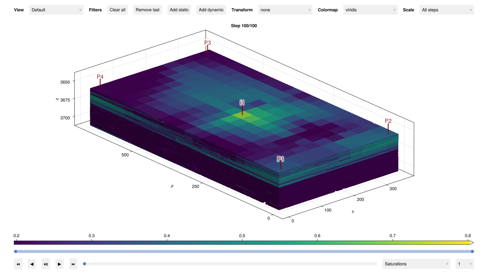

Plot the water cut

using Jutul
t = ws_coarse.time./si_unit(:day)
fig = Figure()
ax = Axis(fig[1, 1]; xlabel = "Time (days)", ylabel = "Water cut")
for w in [:P1, :P2, :P3, :P4]
    wc = ws_coarse[w, :wcut]
    lines!(ax, t, wc; label = "$w")
end
axislegend(position = :lt)
fig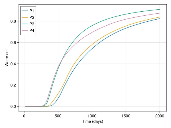

Conclusion

The SPE10, model 2, case is a standard benchmark case for reservoir simulators. JutulDarcy includes premade functions to set up and run this model, including wells, PVT, and the schedule from the original case. The model can be run as-is, or coarsened to a smaller size for testing and development.

Example on GitHub

If you would like to run this example yourself, it can be downloaded from the JutulDarcy.jl GitHub repository as a script, or as a Jupyter Notebook

This example took 195.723089241 seconds to complete.

---

This page was generated using Literate.jl.