Gradient-based optimization of net present value (NPV)
Immiscible InputFile ModelReduction Optimization AdvancedOne usage of a differentiable simulator is control optimization. A counterpart to history matching, control optimization is the process of finding the optimal controls for a given objective and simulation model. In this example, we will optimize the injection rates for a simplified version of the EGG model to maximize the net present value (NPV) of the reservoir.
Setting up a coarse model
We start off by loading the Egg model and coarsening it to a 20x20x3 grid. We limit the optimization to the first 50 timesteps to speed up the optimization process. If you want to run the optimization for all timesteps on the fine model directly, you can remove the slicing of the case and replace the coarse case with the fine case.
using Jutul, JutulDarcy, GLMakie, GeoEnergyIO, LBFGSB
data_dir = GeoEnergyIO.test_input_file_path("EGG")
data_pth = joinpath(data_dir, "EGG.DATA")
fine_case = setup_case_from_data_file(data_pth)
fine_case = fine_case[1:50];
coarse_case = coarsen_reservoir_case(fine_case, (20, 20, 3), method = :ijk);
Set up the rate optimization
We use an utility to set up the rate optimization problem. The utility sets up the objective function, constraints, and initial guess for the optimization. The optimization is set up to maximize the NPV of the reservoir. The contribution to the NPV for a given time
Here,
We set the prices and costs (per barrel) as well as a discount rate of 5% per year. The base rate will be used for all injectors initially, which matches the base case for the Egg model. The utility function takes in a steps argument that can be used to set how often the rates are allowed to change.
The values used here are arbitrary for the purposes of the example. You are encouraged to play around with the values to see how the outcome changes in the optimization. Generally higher discount rates prioritze immediate income, while lower or zero discount rates prioritize maximizing the oil production over the entire simulation period.
ctrl = coarse_case.forces[1][:Facility].control
base_rate = ctrl[:INJECT1].target.value
function optimize_rates(steps; use_box_bfgs = true)
    setup = JutulDarcy.setup_rate_optimization_objective(coarse_case, base_rate,
        max_rate_factor = 10,
        oil_price = 100.0,
        water_price = -10.0,
        water_cost = 5.0,
        discount_rate = 0.05,
        maximize = use_box_bfgs,
        sim_arg = (
            rtol = 1e-5,
            tol_cnv = 1e-5
        ),
        steps = steps
    )
    if use_box_bfgs
        obj_best, x_best, hist = Jutul.unit_box_bfgs(setup.x0, setup.obj,
            maximize = true,
            lin_eq = setup.lin_eq
        )
        H = hist.val
    else
        lower = zeros(length(setup.x0))
        upper = ones(length(setup.x0))
        results, x_best = lbfgsb(setup.F!, setup.dF!, setup.x0,
            lb=lower,
            ub=upper,
            iprint = 1,
            factr = 1e12,
            maxfun = 20,
            maxiter = 20,
            m = 20
        )
        H = results
    end
    return (setup.case, H, x_best)
end
optimize_rates (generic function with 1 method)Optimize the rates
We optimize the rates for two different strategies. The first strategy is to optimize constant rates for the entire period. The second strategy is to optimize the rates for each report step.
Optimize with a single set of rates
case1, hist1, x1 = optimize_rates(:first);Rate optimization: steps=:first selected, optimizing one set of controls for all steps.
Rate optimization: 8 injectors and 4 producers selected.
It. | Objective | Proj. grad | Linesearch-its
-----------------------------------------------
0 | 2.1251e+08 | 1.5242e+08 | -
1 | 2.1992e+08 | 1.0209e+08 | 1
2 | 2.2171e+08 | 4.2945e+07 | 1
3 | 2.2305e+08 | 2.5630e+07 | 1
4 | 2.2387e+08 | 3.4847e+07 | 1
5 | 2.2447e+08 | 2.6204e+07 | 1
6 | 2.2450e+08 | 1.0898e+07 | 2
7 | 2.2451e+08 | 5.8641e+06 | 1
8 | 2.2452e+08 | 6.2265e+06 | 3
LBFGS: Line search unable to succeed in 5 iterations ...
9 | 2.2452e+08 | 6.0429e+06 | 5
10 | 2.2453e+08 | 5.7387e+06 | 2
11 | 2.2454e+08 | 3.8101e+06 | 1
LBFGS: Line search unable to succeed in 5 iterations ...
12 | 2.2454e+08 | 2.2162e+06 | 5
13 | 2.2454e+08 | 2.1549e+06 | 2
14 | 2.2454e+08 | 4.5705e+06 | 2
15 | 2.2454e+08 | 3.1800e+06 | 1
16 | 2.2454e+08 | 2.5527e+06 | 1
17 | 2.2454e+08 | 2.2236e+06 | 1
18 | 2.2454e+08 | 4.0236e+06 | 1
LBFGS: Line search unable to succeed in 5 iterations ...
LBFGS: Hessian not updated during iteration 19
19 | 2.2454e+08 | 2.7160e+06 | 5
LBFGS: Line search unable to succeed in 5 iterations ...
20 | 2.2454e+08 | 2.7790e+06 | 5
LBFGS: Line search unable to succeed in 5 iterations ...
LBFGS: Hessian not updated during iteration 21
21 | 2.2454e+08 | 2.7616e+06 | 5
LBFGS: Line search unable to succeed in 5 iterations ...
22 | 2.2454e+08 | 3.0714e+06 | 5
LBFGS: Line search unable to succeed in 5 iterations ...
23 | 2.2454e+08 | 3.0488e+06 | 5
LBFGS: Line search unable to succeed in 5 iterations ...
24 | 2.2454e+08 | 2.7284e+06 | 5
LBFGS: Line search unable to succeed in 5 iterations ...
25 | 2.2454e+08 | 2.7269e+06 | 5Plot rate allocation for the constant case
fig = Figure()
ax = Axis(fig[1, 1], xlabel = "Injector number", ylabel = "Rate fraction (of max injection rate)")
barplot!(ax, x1)
ax.xticks = eachindex(x1)
fig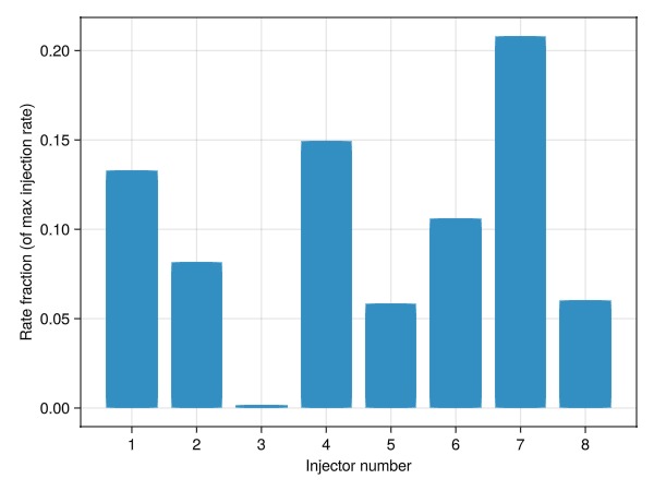
Optimize with varying rates per time-step
case2, hist2, x2 = optimize_rates(:each);Rate optimization: steps=:each selected, optimizing controls for all 50 steps separately.
Rate optimization: 8 injectors and 4 producers selected.
It. | Objective | Proj. grad | Linesearch-its
-----------------------------------------------
0 | 2.1251e+08 | 3.0794e+07 | -
1 | 2.1750e+08 | 6.7921e+06 | 1
2 | 2.1973e+08 | 5.6750e+06 | 1
3 | 2.2229e+08 | 1.0071e+07 | 1
LBFGS: Line search at max step size, Wolfe conditions not satisfied for this step
4 | 2.2237e+08 | 4.0536e+06 | 1
LBFGS: Line search at max step size, Wolfe conditions not satisfied for this step
LBFGS: Hessian not updated during iteration 5
5 | 2.2286e+08 | 2.2465e+06 | 1
6 | 2.2336e+08 | 4.3330e+06 | 2
LBFGS: Line search unable to succeed in 5 iterations ...
7 | 2.2339e+08 | 4.0474e+06 | 5
LBFGS: Line search at max step size, Wolfe conditions not satisfied for this step
LBFGS: Hessian not updated during iteration 8
8 | 2.2358e+08 | 3.9898e+06 | 1
LBFGS: Line search at max step size, Wolfe conditions not satisfied for this step
9 | 2.2366e+08 | 5.4948e+06 | 1
LBFGS: Problematic constraint handling, relative step length: 0.6347257941772806
LBFGS: Line search unable to succeed in 5 iterations ...
10 | 2.2370e+08 | 5.3945e+06 | 5
LBFGS: Problematic constraint handling, relative step length: 0.13974674241482912
11 | 2.2389e+08 | 5.2086e+06 | 1
12 | 2.2419e+08 | 4.8402e+06 | 1
13 | 2.2471e+08 | 4.6890e+06 | 1
LBFGS: Line search unable to succeed in 5 iterations ...
14 | 2.2492e+08 | 5.4159e+06 | 5
LBFGS: Problematic constraint handling, relative step length: 0.4212774023627301
15 | 2.2511e+08 | 6.1346e+06 | 1
16 | 2.2512e+08 | 4.2281e+06 | 1
LBFGS: Problematic constraint handling, relative step length: 0.04046185144482824
LBFGS: Line search unable to succeed in 5 iterations ...
17 | 2.2512e+08 | 4.2091e+06 | 5
LBFGS: Line search unable to succeed in 5 iterations ...
18 | 2.2512e+08 | 4.2194e+06 | 5
LBFGS: Line search unable to succeed in 5 iterations ...
19 | 2.2512e+08 | 4.2194e+06 | 5
20 | 2.2515e+08 | 3.0665e+06 | 2
LBFGS: Line search unable to succeed in 5 iterations ...
LBFGS: Hessian not updated during iteration 21
21 | 2.2516e+08 | 4.0660e+06 | 5
LBFGS: Line search unable to succeed in 5 iterations ...
LBFGS: Hessian not updated during iteration 22
22 | 2.2516e+08 | 4.5969e+06 | 5Plot rate allocation per well
allocs = reshape(x2, length(x1), :)
fig = Figure()
ax = Axis(fig[1, 1], xlabel = "Report step", ylabel = "Rate fraction (of max injection rate)")
for i in axes(allocs, 1)
    lines!(ax, allocs[i, :], label = "Injector #$i")
end
axislegend()
fig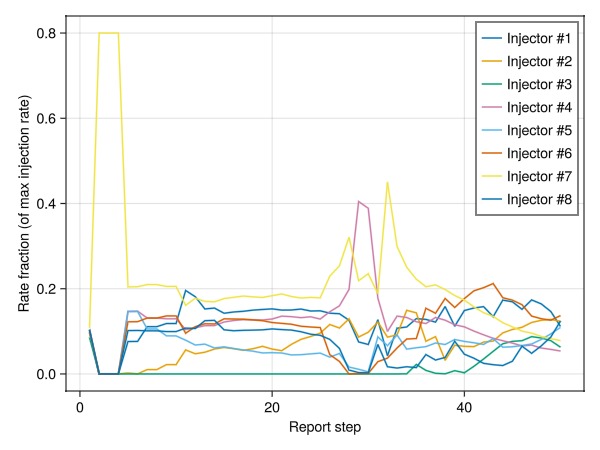
Plot the evolution of the NPV
We plot the evolution of the NPV for the two strategies to compare the results. Note that the optimization produces a higher NPV for the varying rates. This is expected, as the optimization can adjust the rates to the changes in the mobility field during the progress of the simulation.
fig = Figure()
ax = Axis(fig[1, 1], xlabel = "LBFGS iteration", ylabel = "Net present value (million USD)")
scatter!(ax, 1:length(hist1), hist1./1e6, label = "Constant rates")
scatter!(ax, 1:length(hist2), hist2./1e6, marker = :x, label = "Varying rates")
axislegend(position = :rb)
fig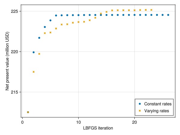
Simulate the results
We finally simulate all the cases to compare the results.
ws0, states0 = simulate_reservoir(coarse_case, info_level = -1)
ws1, states1 = simulate_reservoir(case1, info_level = -1)
ws2, states2 = simulate_reservoir(case2, info_level = -1)
ReservoirSimResult with 50 entries:
wells (12 present):
:PROD4
:INJECT3
:PROD2
:PROD3
:INJECT5
:INJECT4
:INJECT8
:PROD1
:INJECT6
:INJECT1
:INJECT2
:INJECT7
Results per well:
:wrat => Vector{Float64} of size (50,)
:Aqueous_mass_rate => Vector{Float64} of size (50,)
:orat => Vector{Float64} of size (50,)
:bhp => Vector{Float64} of size (50,)
:mrat => Vector{Float64} of size (50,)
:lrat => Vector{Float64} of size (50,)
:mass_rate => Vector{Float64} of size (50,)
:rate => Vector{Float64} of size (50,)
:control => Vector{Symbol} of size (50,)
:Liquid_mass_rate => Vector{Float64} of size (50,)
:wcut => Vector{Float64} of size (50,)
states (Vector with 50 entries, reservoir variables for each state)
:Pressure => Vector{Float64} of size (975,)
:Saturations => Matrix{Float64} of size (2, 975)
:TotalMasses => Matrix{Float64} of size (2, 975)
time (report time for each state)
Vector{Float64} of length 50
result (extended states, reports)
SimResult with 50 entries
extra
Dict{Any, Any} with keys :simulator, :config
Completed at Jul. 10 2026 16:00 after 862 milliseconds, 759 microseconds, 42 nanoseconds.Compute measurables and compare
NPV favors early production, as later income/costs have less relative value. We compute the field measurables to be able to compare the oil and water production.
f0 = reservoir_measurables(coarse_case.model, ws0)
f1 = reservoir_measurables(case1.model, ws1)
f2 = reservoir_measurables(case2.model, ws2)
Dict{Symbol, Any} with 19 entries:
:fwit => (values = [636.0, 1370.93, 2450.5, 5077.41, 11030.9, 17336.4, 23696.…
:fwpt => (values = [0.34967, 0.349671, 0.349671, 0.349671, 0.349671, 0.349671…
:flpr => (values = [0.0071688, 0.00215896, 0.00248597, 0.00303579, 0.00689591…
:time => [86400.0, 432000.0, 864000.0, 1.728e6, 2.592e6, 3.456e6, 4.32e6, 5.1…
:fwct => (values = [0.000564544, 1.46667e-9, 1.70915e-13, 4.36241e-18, 1.3140…
:fopr => (values = [0.00716475, 0.00215896, 0.00248597, 0.00303579, 0.0068959…
:fwir => (values = [0.00736111, 0.00212654, 0.00249899, 0.00304041, 0.0068906…
:foir => (values = [0.0, 0.0, 0.0, 0.0, 0.0, 0.0, 0.0, 0.0, 0.0, 0.0 … 0.0,…
:flir => (values = [0.0, 0.0, 0.0, 0.0, 0.0, 0.0, 0.0, 0.0, 0.0, 0.0 … 0.0,…
:fgpr => (values = [0.0, 0.0, 0.0, 0.0, 0.0, 0.0, 0.0, 0.0, 0.0, 0.0 … 0.0,…
:fgir => (values = [0.0, 0.0, 0.0, 0.0, 0.0, 0.0, 0.0, 0.0, 0.0, 0.0 … 0.0,…
:fwpr => (values = [4.0471e-6, 3.16649e-12, 4.24891e-16, 1.32434e-20, 9.06175…
:fgit => (values = [0.0, 0.0, 0.0, 0.0, 0.0, 0.0, 0.0, 0.0, 0.0, 0.0 … 0.0,…
:fgor => (values = [0.0, 0.0, 0.0, 0.0, 0.0, 0.0, 0.0, 0.0, 0.0, 0.0 … 0.0,…
:flit => (values = [0.0, 0.0, 0.0, 0.0, 0.0, 0.0, 0.0, 0.0, 0.0, 0.0 … 0.0,…
:fopt => (values = [619.035, 1365.17, 2439.11, 5062.04, 11020.1, 17321.7, 236…
:foit => (values = [0.0, 0.0, 0.0, 0.0, 0.0, 0.0, 0.0, 0.0, 0.0, 0.0 … 0.0,…
:fgpt => (values = [0.0, 0.0, 0.0, 0.0, 0.0, 0.0, 0.0, 0.0, 0.0, 0.0 … 0.0,…
:flpt => (values = [619.384, 1365.52, 2439.46, 5062.39, 11020.5, 17322.0, 236…Plot the cumulative field oil production
The optimized cases produce more oil than the base case.
bbl = si_unit(:stb)
fig = Figure()
ax = Axis(fig[1, 1], xlabel = "Time / days", ylabel = "Field oil production (accumulated, barrels)", title = "Base case")
t = ws0.time./si_unit(:day)
lines!(ax, t, f0[:fopt].values./bbl, label = "Base case")
lines!(ax, t, f1[:fopt].values./bbl, label = "Constant rates")
lines!(ax, t, f2[:fopt].values./bbl, label = "Varying rates")
axislegend(position = :rb)
fig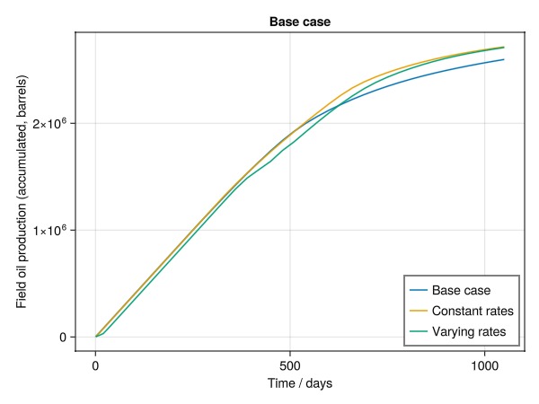
Plot the cumulative field water production
The optimized cases produce less water than the base case.
fig = Figure()
ax = Axis(fig[1, 1], xlabel = "Time / days", ylabel = "Field water production (accumulated, barrels)", title = "Base case")
t = ws0.time./si_unit(:day)
lines!(ax, t, f0[:fwpt].values./bbl, label = "Base case")
lines!(ax, t, f1[:fwpt].values./bbl, label = "Constant rates")
lines!(ax, t, f2[:fwpt].values./bbl, label = "Varying rates")
axislegend(position = :rb)
fig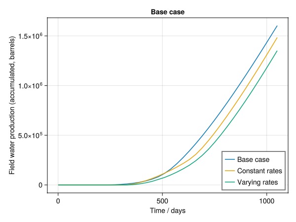
Plot the differences in water saturation
The optimized cases have a different water saturation distribution compared to the base case.
reservoir = reservoir_domain(coarse_case.model)
g = physical_representation(reservoir)
function plot_diff!(ax, s)
    plt = plot_cell_data!(ax, g, s0 - s1, colorrange = (-0.5, 0.5), colormap = :balance)
    for (w, wd) in get_model_wells(coarse_case.model)
        plot_well!(ax, g, wd, top_factor = 0.8, fontsize = 10)
    end
    ax.elevation[] = 1.03
    ax.azimuth[] = 3.75
    return plt
end

s0 = states0[end][:Saturations][1, :]
s1 = states1[end][:Saturations][1, :]
s2 = states2[end][:Saturations][1, :]
fig = Figure(size = (1600, 800))
ax = Axis3(fig[1, 1], zreversed = true, title = "Water saturation difference, constant rates")
plt = plot_diff!(ax, s1)
ax = Axis3(fig[1, 2], zreversed = true, title = "Water saturation difference, varying rates")
plot_diff!(ax, s2)
Colorbar(fig[2, :], plt, vertical = false)
fig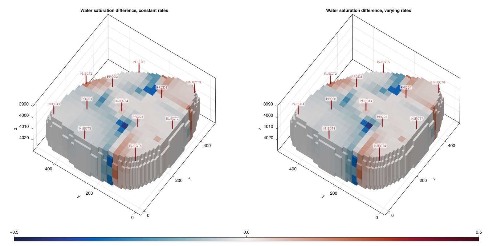
Example on GitHub
If you would like to run this example yourself, it can be downloaded from the JutulDarcy.jl GitHub repository as a script
This example took 334.369997844 seconds to complete.This page was generated using Literate.jl.