Geothermal doublet
Geothermal IntroductionThis example demonstrates how to set up a geothermal doublet simulation using JutulDarcy. We will use two different PVT functions–one simple and one realistic–to highlight the importance of accurate fluid physics in geothermal simulations.
using Jutul, JutulDarcy, GeoEnergyIO, GLMakie
meter, kilogram, bar, year = si_units(:meter, :kilogram, :bar, :year)
(1.0, 1.0, 100000.0, 3.1556952e7)Make setup function
We use the synthethic EGG model [8] to emulate realistic geology. Instead of using the original wells, we set up a simple injector-producer doublet, placed so that injected fluids will sweep a large part of the reservoir.
Set up EGG model
egg_dir = JutulDarcy.GeoEnergyIO.test_input_file_path("EGG")
data_pth = joinpath(egg_dir, "EGG.DATA")
case0 = setup_case_from_data_file(data_pth)
domain = reservoir_model(case0.model).data_domain;
Make setup function
function setup_doublet(sys)

    inj_well = setup_vertical_well(domain, 45, 15, name = :Injector, simple_well = false)
    prod_well = setup_vertical_well(domain, 15, 45, name = :Producer, simple_well = false)

    model = setup_reservoir_model(
        domain, sys,
        thermal = true,
        wells = [inj_well, prod_well],
    );
    rmodel = reservoir_model(model)
    push!(rmodel.output_variables, :PhaseMassDensities, :PhaseViscosities)

    state0 = setup_reservoir_state(model,
        Pressure = 50bar,
        Temperature = convert_to_si(90, :Celsius)
    )

    time = 50year
    pv_tot = sum(pore_volume(reservoir_model(model).data_domain))
    rate = 2*pv_tot/time
    rate_target = TotalRateTarget(rate)
    ctrl_inj  = InjectorControl(rate_target, [1.0],
        density = 1000.0, temperature = convert_to_si(10.0, :Celsius))

    bhp_target = BottomHolePressureTarget(25bar)
    ctrl_prod = ProducerControl(bhp_target)

    control = Dict(:Injector => ctrl_inj, :Producer => ctrl_prod)

    dt = 4year/12
    dt = fill(dt, Int(time/dt))

    forces = setup_reservoir_forces(model, control = control)

    return JutulCase(model, dt, forces, state0 = state0)

end
setup_doublet (generic function with 1 method)Simple fluid physics
We start by setting up a simple fluid physics where water is slightly compressible, but with no influence of temperature. Viscosity is constant.
rhoWS = 1000.0kilogram/meter^3
sys = SinglePhaseSystem(AqueousPhase(), reference_density = rhoWS)
case_simple = setup_doublet(sys)
results_simple = simulate_reservoir(case_simple);
Jutul: Simulating 50 years as 150 report steps
╭────────────────┬───────────┬───────────────┬──────────╮
│ Iteration type │ Avg/step │ Avg/ministep │ Total │
│ │ 150 steps │ 156 ministeps │ (wasted) │
├────────────────┼───────────┼───────────────┼──────────┤
│ Newton │ 1.14667 │ 1.10256 │ 172 (0) │
│ Linearization │ 2.18667 │ 2.10256 │ 328 (0) │
│ Linear solver │ 2.33333 │ 2.24359 │ 350 (0) │
│ Precond apply │ 4.66667 │ 4.48718 │ 700 (0) │
╰────────────────┴───────────┴───────────────┴──────────╯
╭───────────────┬──────────┬────────────┬─────────╮
│ Timing type │ Each │ Relative │ Total │
│ │ ms │ Percentage │ s │
├───────────────┼──────────┼────────────┼─────────┤
│ Properties │ 0.7022 │ 0.54 % │ 0.1208 │
│ Equations │ 33.5299 │ 49.20 % │ 10.9978 │
│ Assembly │ 2.4064 │ 3.53 % │ 0.7893 │
│ Linear solve │ 2.4493 │ 1.88 % │ 0.4213 │
│ Linear setup │ 24.0351 │ 18.49 % │ 4.1340 │
│ Precond apply │ 1.6688 │ 5.23 % │ 1.1682 │
│ Update │ 2.8665 │ 2.21 % │ 0.4930 │
│ Convergence │ 5.9305 │ 8.70 % │ 1.9452 │
│ Input/Output │ 1.5006 │ 1.05 % │ 0.2341 │
│ Other │ 11.9225 │ 9.17 % │ 2.0507 │
├───────────────┼──────────┼────────────┼─────────┤
│ Total │ 129.9674 │ 100.00 % │ 22.3544 │
╰───────────────┴──────────┴────────────┴─────────╯Interactive plot of the reservoir state
plot_reservoir(case_simple.model, results_simple.states)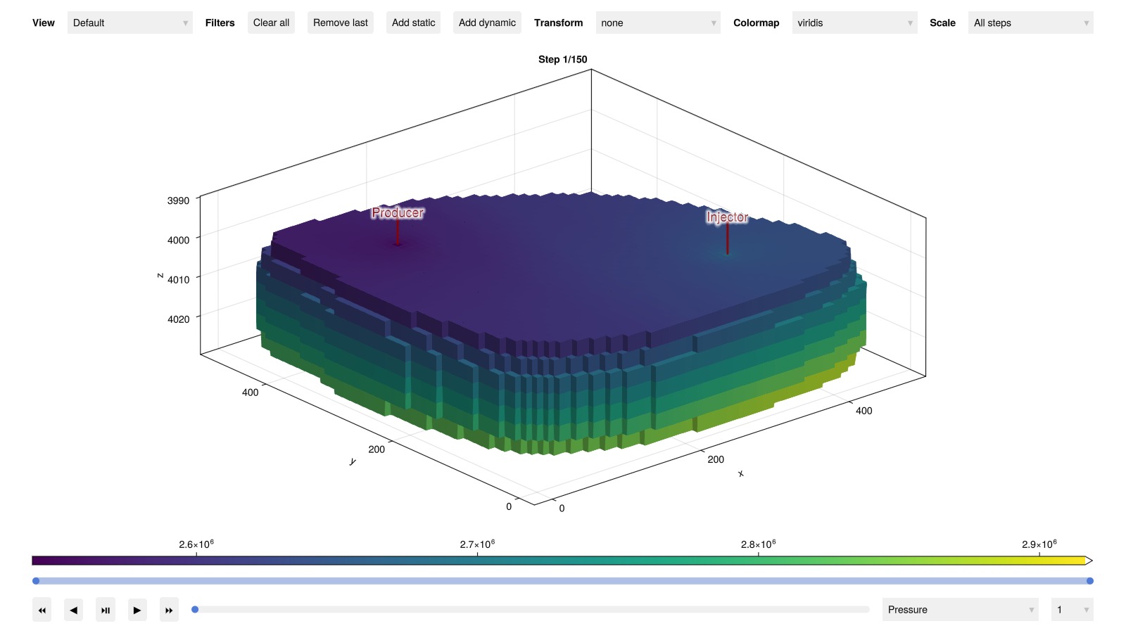
Realistic fluid physics
Next, we repeat the simulation with more realistic fluid physics. We use a formulation from NIST where density, viscosity and heat capacity depend on pressure and temperature.
case_real = setup_doublet(:geothermal)
results_real = simulate_reservoir(case_real);
Jutul: Simulating 50 years as 150 report steps
╭────────────────┬───────────┬───────────────┬──────────╮
│ Iteration type │ Avg/step │ Avg/ministep │ Total │
│ │ 150 steps │ 157 ministeps │ (wasted) │
├────────────────┼───────────┼───────────────┼──────────┤
│ Newton │ 2.21333 │ 2.11465 │ 332 (0) │
│ Linearization │ 3.26 │ 3.11465 │ 489 (0) │
│ Linear solver │ 8.03333 │ 7.67516 │ 1205 (0) │
│ Precond apply │ 16.0667 │ 15.3503 │ 2410 (0) │
╰────────────────┴───────────┴───────────────┴──────────╯
╭───────────────┬─────────┬────────────┬─────────╮
│ Timing type │ Each │ Relative │ Total │
│ │ ms │ Percentage │ s │
├───────────────┼─────────┼────────────┼─────────┤
│ Properties │ 1.8453 │ 3.31 % │ 0.6126 │
│ Equations │ 8.2054 │ 21.67 % │ 4.0124 │
│ Assembly │ 1.5406 │ 4.07 % │ 0.7534 │
│ Linear solve │ 2.7226 │ 4.88 % │ 0.9039 │
│ Linear setup │ 23.2486 │ 41.68 % │ 7.7185 │
│ Precond apply │ 1.6537 │ 21.52 % │ 3.9853 │
│ Update │ 0.4589 │ 0.82 % │ 0.1523 │
│ Convergence │ 0.3639 │ 0.96 % │ 0.1779 │
│ Input/Output │ 0.4147 │ 0.35 % │ 0.0651 │
│ Other │ 0.4167 │ 0.75 % │ 0.1384 │
├───────────────┼─────────┼────────────┼─────────┤
│ Total │ 55.7829 │ 100.00 % │ 18.5199 │
╰───────────────┴─────────┴────────────┴─────────╯Interactive plot of the reservoir state
plot_reservoir(case_real.model, results_real.states)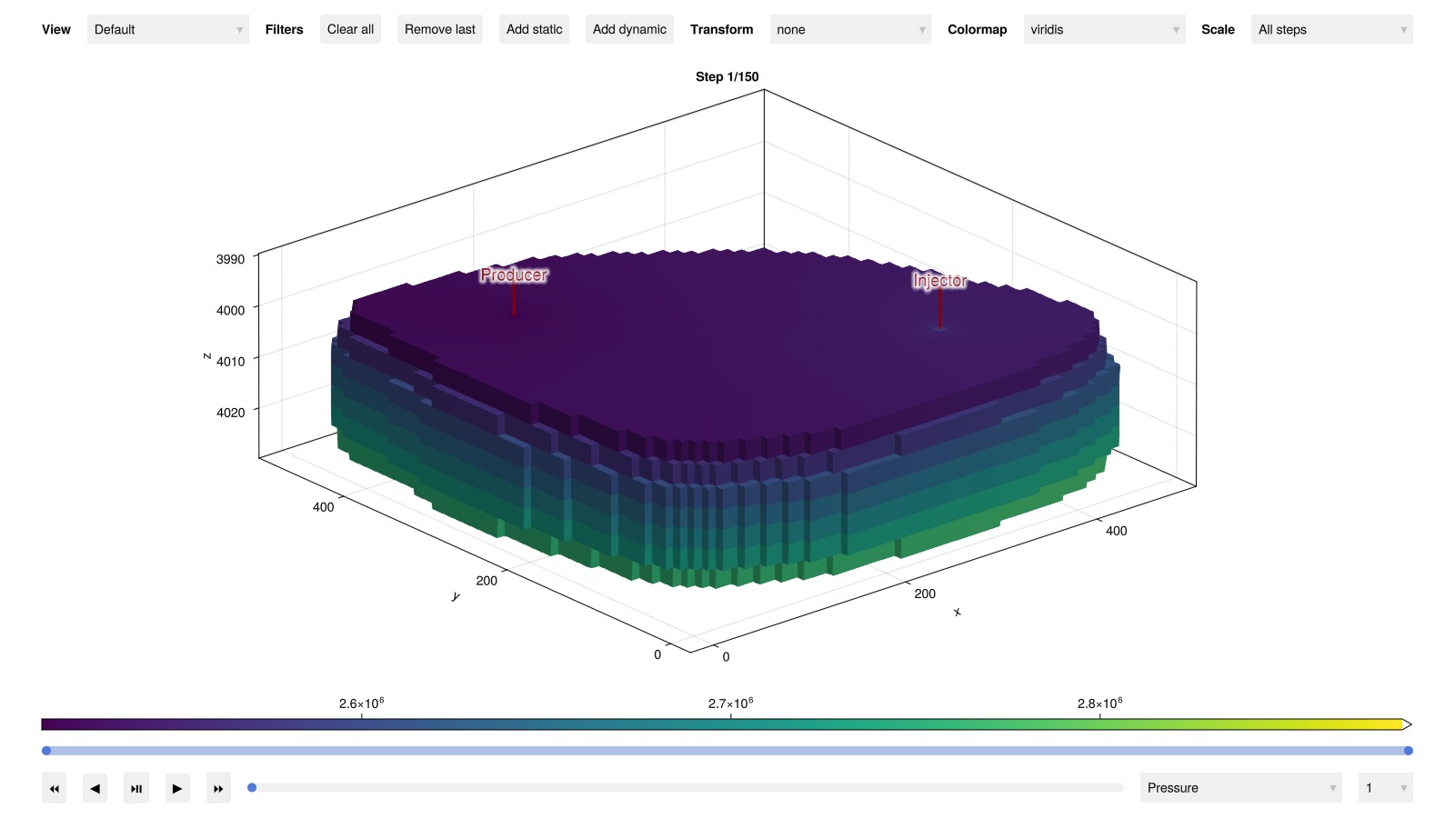
Compare results
A key performace metric for geothermal doublets is the time it takes before the cold water injected to uphold pressure reaches the producer. At this point, production temperature will rapidly decline, so that the breakthrough time effectively defines the lifespan of the doublet. We plot the well results for the two simulations to compare the two different PVT formulations. Since water viscosty is not affected by temperature in the simple PVT model, water movement is much faster in this scenario, thereby grossly underestimating the lifespan of the doublet compared to the realistic PVT. This effect is further amplified by the thermal shrinkage due to colling present in the realistic PVT model.
plot_well_results([results_simple.wells, results_real.wells]; names = ["Simple", "Realistic"])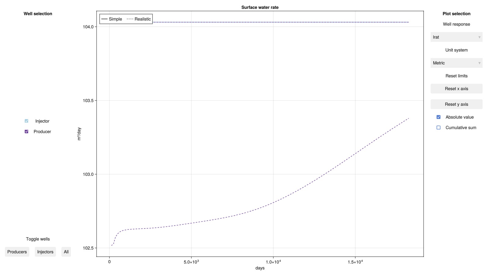
Finally, we plot the density to see how the two simulations differ. As density in the the simple PVT is only dependent on pressure, it is largely constant except from in the vicinity of the wells, where pressure gradients are larger. In the realistic PVT, where density is a function of both pressure and temperature, we see that it is affected in all regions swept by the injected cold water.
ρ_simple = map(s -> s[:PhaseMassDensities], results_simple.states)
ρ_real = map(s -> s[:PhaseMassDensities], results_real.states)
Δρ = map(Δρ -> Dict(:DensityDifference => Δρ), ρ_simple .- ρ_real)
plot_reservoir(case_real.model, Δρ; step = length(Δρ))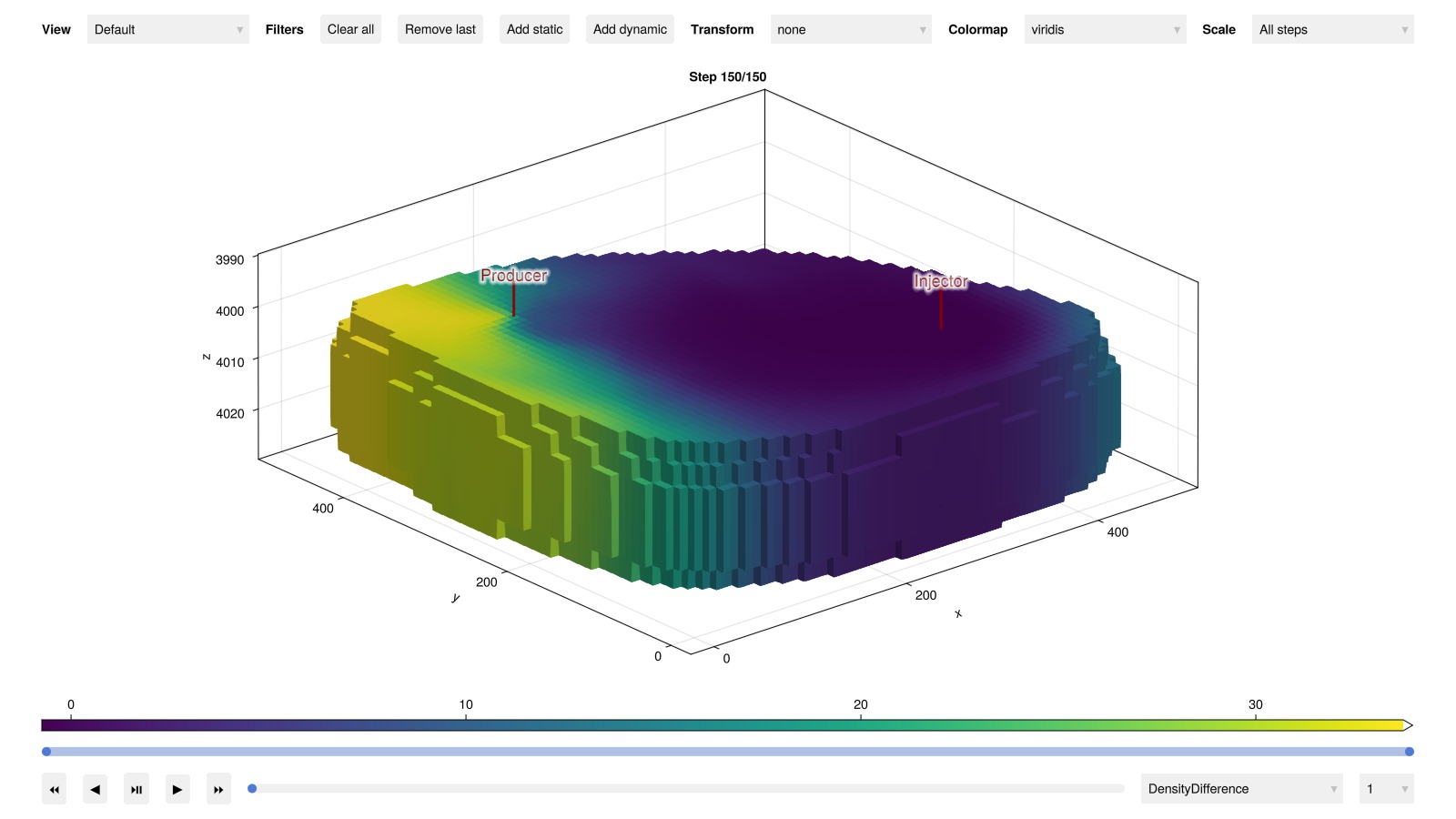
Example on GitHub
If you would like to run this example yourself, it can be downloaded from the JutulDarcy.jl GitHub repository as a script
This example took 68.277442722 seconds to complete.This page was generated using Literate.jl.