Hydrostatic equilibriation of models
Immiscible Compositional Blackoil IntroductionInitializing a reservoir model is an important part of reservoir simulation. For simple, conceptual models it may be sufficient to prescribe a single uniform pressure value as the initial condition, but for more realistic cases the problem of equilibriation becomes very important.
This example gives an overview of how to set up the initial state of a reservoir model using the setup_reservoir_state function. To set up a reservoir model, values for all primary variables must be provided for every cell of the domain. The wells are automatically initialized from the cell values. There are two main ways the initial state can be set up:
Direct assignment, where the initial values are provided directly as either values for one cell, or values for all cells in the domain. This has the advantage of being very easy to set up, and gives you full control over the initial conditions, but it can be difficult to set up realistic initial that correspond to hydrostatic equilibrium. This means that the model can have significant mass transfer between cells starting from the initial conditions even without wells or boundary conditions.
Equilibriation, where the initial values are computed from a set of ordinary differential equations that makes sure the initial state is in hydrostatic equilibrium. This is the most realistic way to set up the initial conditions, but requires additional inputs.
We will go over both of these approaches in this example. The corresponding terminology from typical input files would be keywords like EQUIL (for hydrostatic equilibriation) and PRES, SGAS, SOIL and so on (for direct assignment). If an input file is used, the initial state will set up automatically from these keywords.
using Jutul, JutulDarcy, MultiComponentFlash, GLMakie, GeoEnergyIOSet up a reservoir with depth for the examples
We will use a simple Cartesian mesh with 2 cells in the x-direction and 1000 cells in the z-direction. The domain is 20 m wide, 10 m high and 1000 m deep. Note that we set z_is_depth = true to make sure the z coordinate is treated as depth, which is customary for resrvoir models, and assumed by the functions that set up the initial state based on hydrostatic equilibrium. We also shift the mesh so that the top of the domain is at 800 m depth.
nx = 2
nz = 1000
Darcy, bar, yr, Kelvin = si_units(:darcy, :bar, :year, :Kelvin)
cmesh = reservoir_mesh((nx, 1, nz), (20.0, 10.0, 1000.0))
for (i, pt) in enumerate(cmesh.node_points)
    cmesh.node_points[i] = pt .+ [0.0, 0.0, 800.0]
end
reservoir = reservoir_domain(cmesh, porosity = 0.25, permeability = 0.1*Darcy)
ncells = number_of_cells(cmesh)2000Set up a three-phase model with simple initial conditions
We will start by setting up a three-phase model with simple initial conditions. We let the initial conditions be uniform throughout the domain. This is done by passing a scalar for the pressure (which will be repeated for all cells) and a vector with one entry per hphase for the saturations (which will be repeated for all cells into a 3 by ncells matrix).
We also set a typical density function. The density function is important, as it determines the pressure distribution for the equilibrium state.
W = AqueousPhase()
O = LiquidPhase()
G = VaporPhase()

rhoS = [1000.0, 700.0, 100.0]
sys_3ph = ImmiscibleSystem((W, O, G), reference_densities = rhoS)
rho = ConstantCompressibilityDensities(sys_3ph, 1.5bar, rhoS, 1e-5/bar)
model_3ph = setup_reservoir_model(reservoir, sys_3ph)
set_secondary_variables!(model_3ph[:Reservoir], PhaseMassDensities = rho)
state0_3ph_1 = setup_reservoir_state(model_3ph, Saturations = [0.0, 1.0, 0.0], Pressure = 200*bar)
Dict{Any, Any} with 1 entry:
:Reservoir => Dict{Symbol, Any}(:PhaseMassMobilities=>[0.0 0.0 … 0.0 0.0; 0.0…Simulate the model and plot the change in pressure
We will now simulate the model for 100 years and plot the change in pressure. This could be thought of as the poor man's way of setting up the initial state, as it will give a pressure distribution that is close to hydrostatic equilibrium at the cost of solving many time-steps. For a small model, this cost is negligble, but for larger models it can be significant.
We observe that the initially constant pressure becomes a nearly linear function of depth after 100 years. This is the expected result for a model with constant and no driving forces other than gravity.
dt = [convert_to_si(100, :year)]
_, states_3ph_1 = simulate_reservoir(state0_3ph_1, model_3ph, dt)

function plot_comparison(v1, v2, t)
    clim = extrema([v1..., v2...])
    fig = Figure(size = (1000, 500))
    to_mesh(x) = reshape(x, nx, nz)[:, end:-1:1]
    ax1 = Axis(fig[1, 1], title = "$t initial condition")
    heatmap!(ax1, to_mesh(v1), colorrange = clim, colormap = :coolwarm)
    ax2 = Axis(fig[1, 2], title = "$t after 100 years")
    plt = heatmap!(ax2, to_mesh(v2), colorrange = clim, colormap = :coolwarm)
    Colorbar(fig[1, 3], plt)
    fig
end
plot_comparison(state0_3ph_1[:Reservoir][:Pressure]./bar, states_3ph_1[1][:Pressure]./bar, "Pressure [bar]")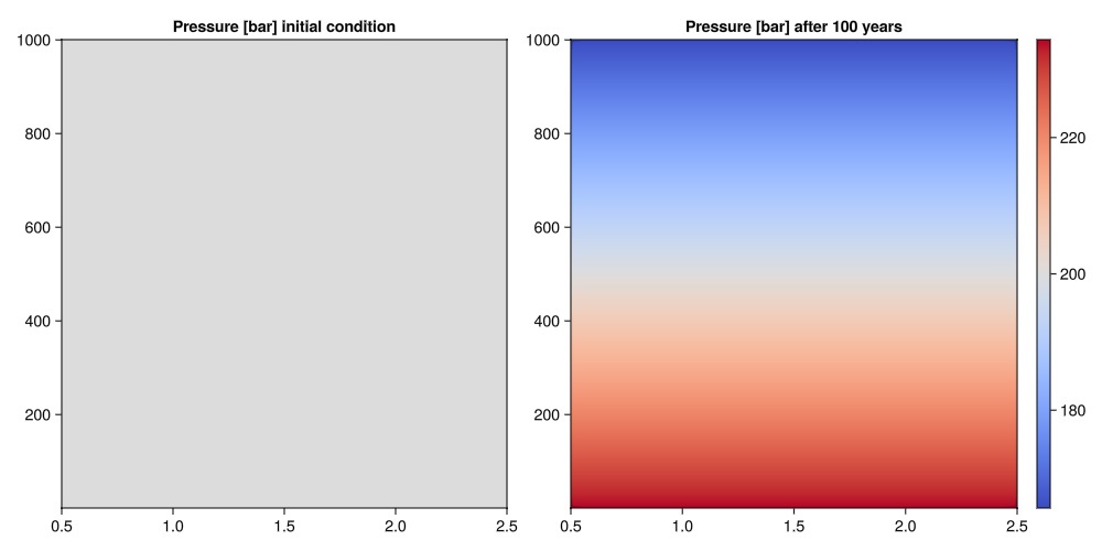
Confirm that the pressure distribution is approximately linear
The pressure should follow the hydrostatic pressure distribution, i.e. for a single-phase initial state it would be the solution of the ODE:
Note that as when the variation of the density with respect to pressure is small, this is essentially saying that:
function pressure_vs_depth_plot(state)
    if haskey(state, :Reservoir)
        state = state[:Reservoir]
    end
    p = state[:Pressure]./bar
    z = reservoir[:cell_centroids][3, :]
    fig = Figure(size = (300, 600))
    ax = Axis(fig[1, 1], title = "Pressure vs depth", ylabel = "Depth [m]", xlabel = "Pressure [bar]")
    plt = scatter!(ax, p, z, color = p, markersize = 2, colormap = :coolwarm)
    Colorbar(fig[1, 2], plt)
    fig
end
pressure_vs_depth_plot(states_3ph_1[end])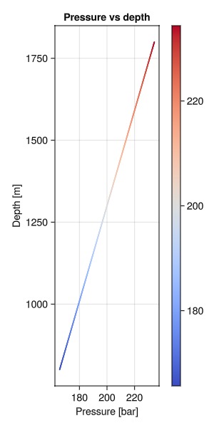
Initialize the model with random initial conditions
We will now set up the model with random initial conditions by providing values per cell. This is done by providing a vector with one entry per cell for pressure, taking care to avoid zero or negative pressures. Similarily, the saturations can be provided as a 3 by ncells matrix, taking care to ensure that the sum of the saturations is equal to one in each cell (i.e. each column of the matrix). This will also return to a hydrostatic distribution, but the saturations make the results more interesting.
s0 = 0.2 .+ rand(3, ncells)
s0 = s0 ./ sum(s0, dims = 1)
p0 = 100 .* (0.1 .+ rand(ncells)).*bar
state0_3ph_rand = setup_reservoir_state(model_3ph, Saturations = s0, Pressure = p0)
_, states_3ph_rand = simulate_reservoir(state0_3ph_rand, model_3ph, dt)
plot_comparison(p0./bar, states_3ph_rand[1][:Pressure]./bar, "Pressure [bar]")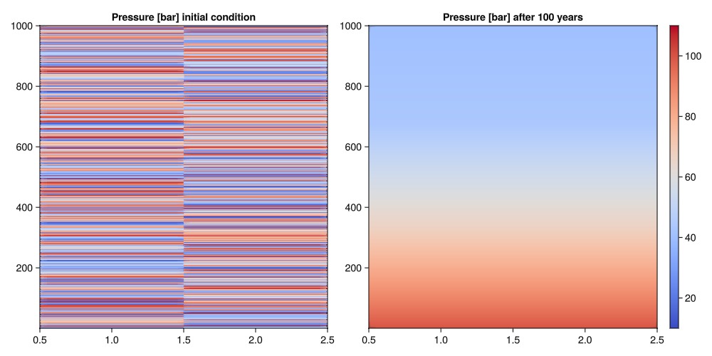
Plot the water saturation
We will now plot the water saturation for the initial condition and the state after 100 years. We observe that the initially random water saturation migrates to the bottom of the model. This is expected, as the water is the heaviest phase. A similar observation could be made for the other two phases.
plot_comparison(s0[1, :], states_3ph_rand[1][:Saturations][1, :], "Water saturation")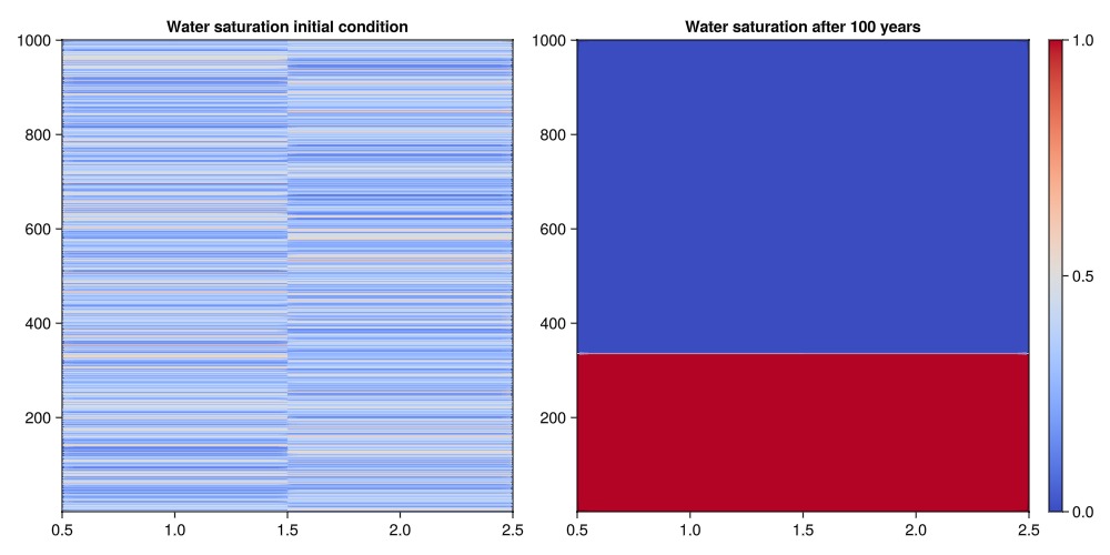
Plot the pressure distribution for the random initial condition
We now observe a bit more interesting pressure distribution. The slope of the pressure gradient is still linear, but the slope varies in three different regions: One for the top region where gas/vapor migrates, one for the middle region where oil/liquid migrates and one for the bottom region where water migrates.
pressure_vs_depth_plot(states_3ph_rand[end])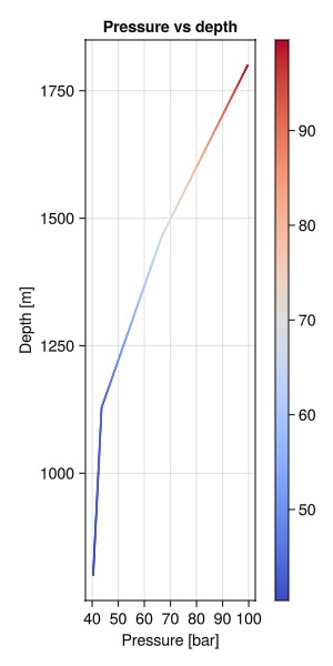
Equilibriate the model
We will now set up the model with a more realistic initial condition by equilibriating the model. This is done by providing a set of parameters that describe the equilibrium state. The most important parameter is the pressure at a given depth (datum depth and pressure) which fixes the pressure range in the model. In addition, we provide the depths of the fluid contacts where pairs of phases are in contact with each other at hydrostatic equilibrium.
eql = EquilibriumRegion(model_3ph, 100*bar, 1000.0, woc = 1600.0, goc = 1100.0)EquilibriumRegion{Float64} for 2000 cells with datum pressure 1.0e7 Pa at depth 1000.0 m
Water-Oil Contact: 1600.0 m, Gas-Oil Contact: 1100.0 m, Water-Gas Contact: NaN mPerform equilibriation
We simply pass the equilibrium region to the setup_reservoir_state function as a second positional argument.
state0_3_ph_eql = setup_reservoir_state(model_3ph, eql)Dict{Any, Any} with 1 entry:
:Reservoir => Dict{Symbol, Any}(:PhaseMassMobilities=>[0.0 0.0 … 0.0 0.0; 0.0…Plot the results
We plot the initial condition of the pressure (left) and the saturations (right).
function plot_state0(state, phases = :wog)
    has_sat = haskey(state[:Reservoir], :Saturations)
    has_comp = haskey(state[:Reservoir], :OverallMoleFractions)
    fig = Figure(size = ((1 + has_sat + has_comp)*300, 500))
    to_mesh(x) = reshape(x, nx, nz)[:, end:-1:1]
    ax1 = Axis(fig[1, 1], title = "Pressure")
    p = state[:Reservoir][:Pressure]./si_unit(:bar)
    plt_pres = heatmap!(ax1, to_mesh(p), colormap = :coolwarm)
    Colorbar(fig[1, 2], plt_pres)

    if has_sat
        sat = state[:Reservoir][:Saturations]
        function to_rgb(i)
            if phases == :wog
                return Makie.RGB(sat[2, i], sat[3, i], sat[1, i])
            elseif phases == :og
                return Makie.RGB(sat[1, i], sat[2, i], 0.0)
            elseif phases == :wg
                return Makie.RGB(0.0, sat[2, i], sat[1, i])
            end
        end
        sat_rgb = map(to_rgb, axes(sat, 2))
        ax2 = Axis(fig[1, 3], title = "Saturation")
        plt = heatmap!(ax2, to_mesh(sat_rgb), colormap = :coolwarm)

        e_wat = PolyElement(color = Makie.RGB(0.0, 0.0, 1.0), strokecolor = :black, strokewidth = 1)
        e_oil = PolyElement(color = Makie.RGB(1.0, 0.0, 0.0), strokecolor = :black, strokewidth = 1)
        e_gas = PolyElement(color = Makie.RGB(0.0, 1.0, 0.0), strokecolor = :black, strokewidth = 1)

        Legend(fig[1, 4],
        [e_wat, e_oil, e_gas],
        ["Aqeous (W)", "Liquid (O)", "Vapor (G)"],
        patchsize = (35, 35), rowgap = 10)
        if has_comp
            comp = state[:Reservoir][:OverallMoleFractions]
            ax3 = Axis(fig[1, 5], title = "Mole fraction, component 1")
            plt_comp = heatmap!(ax3, to_mesh(comp[1, :]), colorrange = (0.0, 1.0))
            Colorbar(fig[1, 6], plt_comp)
        end
    end
    fig
end
plot_state0(state0_3_ph_eql)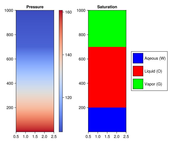
Plot the pressure distribution by depth
pressure_vs_depth_plot(state0_3_ph_eql)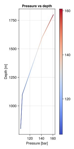
Set up a two-region model
We can also easily set up two different regions in the model. This is done by providing a vector of cell indices for each region, and then passing the vector if regions to the setup_reservoir_state. Each region can also be associated with a separate PVT or saturation region.
Note that if the regions are in pressure contact (i.e. there is no flow barrier between them), this state will not be a true equilibrium state and the fluids will move between the regions when simulation starts. The primary utility of setting up multiple regions is to simulate compartments that have different contacts in the same model, for example because a well passes through both compartments.
A = Int[]
B = Int[]
for c in 1:ncells
    I, J, K = cell_ijk(cmesh, c)
    if I == 1
        push!(A, c)
    else
        push!(B, c)
    end
end
eql_A = EquilibriumRegion(model_3ph, 100*bar, 1000.0, woc = 1600.0, goc = 1100.0, cells = A)
eql_B = EquilibriumRegion(model_3ph, 120*bar, 1000.0, woc = 1500.0, goc = 1200.0, cells = B)
state0_two_reg = setup_reservoir_state(model_3ph, [eql_A, eql_B])
plot_state0(state0_two_reg)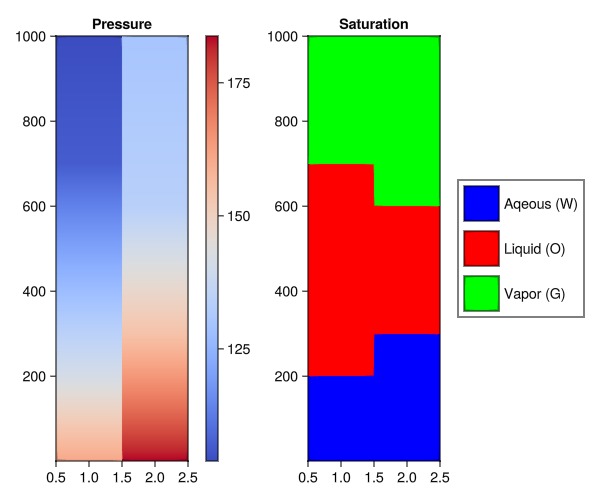
The two regions are easy to see in a scatter plot
pressure_vs_depth_plot(state0_two_reg)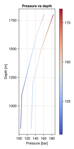
Load a black-oil model with capillary pressure
We load the SPE9 model and transfer the fluid system over to our small reservoir model to see how equilibrium can be computed for a black-oil model.
spe9 = GeoEnergyIO.test_input_file_path("SPE9", "SPE9.DATA");
case = setup_case_from_data_file(spe9)
model_bo = setup_reservoir_model(reservoir, case.model);
PVT: Fixing table for low pressure conditions.Equilibriate the model
We will now equilibriate the black-oil model. Note that we can specify the Rs value by depth. The density of the liquid phase in this model depends on the dissolved gas. Changing the Rs value will change the density of the liquid phase, which will in turn change the pressure distribution. Rs can be specified using either rs (constant value) or rs_vs_depth (function of depth). For models with vaporized oil, a similar pair of options is present for Rv.
Note that the oil saturation is not uniform in the oil region, as there is a capillary fringe present. This is a common feature in black-oil models, where significant capillary pressure between the oil and water phases can lead to significant water being "pulled up" into the oil region against the force of gravity until the two effects balance out.
eql_bo = EquilibriumRegion(model_bo, 100*bar, 1000.0, woc = 1600.0, goc = 1100.0, rs = 15.0)
state0_bo = setup_reservoir_state(model_bo, eql_bo)
plot_state0(state0_bo)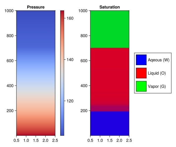
See the effect of capillary pressure on the pressure distribution
The capillary equilibrium will be accounted. We can see this effect in detail by plotting the capillary pressure and the water saturation by depth. Note that there is connate water in the oil and gas regions, and variation within the oil zone.
pc = model_bo[:Reservoir][:CapillaryPressure].pc[1][1] # WO pc, first region
krw = model_bo[:Reservoir][:RelativePermeabilities].krw[1] # WO pc, first region
sw = state0_bo[:Reservoir][:Saturations][1, :]
fig = Figure(size = (1000, 500))
ax1 = Axis(fig[1, 1], title = "Water-Oil capillary pressure", ylabel = "Capillary pressure [bar]")
plt_pc = lines!(ax1, pc.X, pc.F./bar)
ax2 = Axis(fig[1, 2], title = "Water saturation by depth", ylabel = "Depth [m]", xlabel = "Saturation")
plt_sw = lines!(ax2, sw, reservoir[:cell_centroids][3, :])
ax3 = Axis(fig[1, 3], title = "Water-Oil relative permeability", ylabel = "Kr", xlabel = "Water saturation")
plt_krw = lines!(ax3, krw.k.X, krw.k.F)
fig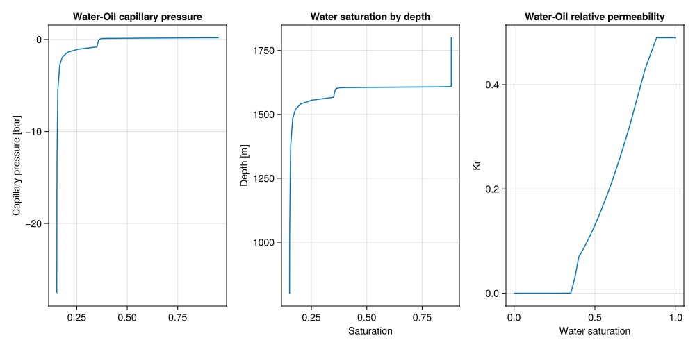
Scaled capillary pressure
We can also perform cell-by-cell scaling of the capillary pressure. This is done by providing a matrix of scaling factors for the capillary pressure, which will be multiplied with the capillary pressure function on a cell-by-cell basis. This can be used to model heterogeneity in the capillary pressure, for example due to variations in pore size distribution or wettability. The scaling factors can be provided as a keyword argument to set_capillary_pressure!, and will be stored in the reservoir domain under the key :capillary_pressure_scaling.
We set up capillary pressure manually by taking the SPE9 SWOF/SGOF tables and then applying uniform scaling per curve.
model_bo_scaled = setup_reservoir_model(deepcopy(reservoir), case.model);
props = case.input_data["PROPS"]
swof = props["SWOF"][1]
sgof = props["SGOF"][1]
scaling = ones(2, number_of_cells(reservoir))
scaling[1, :] .= 10.0
set_capillary_pressure!(model_bo_scaled, pcow = swof, pcog = sgof, cell_scaling = scaling)
state0_bo_scaled = setup_reservoir_state(model_bo_scaled, eql_bo)
plot_state0(state0_bo_scaled)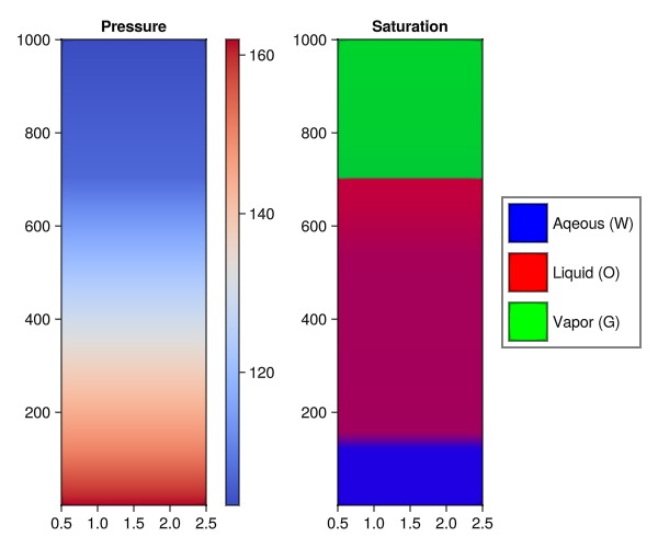
Set up a compositional model
We will now set up a compositional model with two components. The components are methane (will mostly form a gas) and n-decane (will mostly be liquid).
c_light = MolecularProperty("Methane")
c_heavy = MolecularProperty("n-Decane")
mixture = MultiComponentMixture([c_light, c_heavy])
eos = GenericCubicEOS(mixture, PengRobinson())
sys_c = MultiPhaseCompositionalSystemLV(eos, (LiquidPhase(), VaporPhase()))
model_comp = setup_reservoir_model(reservoir, sys_c);
Equilibriate the model
We will now equilibriate the compositional model. The compositional model can be equilibrated in much the same manner, but unlike the previous model two models, there are additional requirements on the inputs. Compositional models predict the density and phase saturations based on the composition and temperature and thus specifying composition and temperature as a function of depth is mandatory.
It is important that the compositions are consistent with the phase behavior, i.e. specifying a composition that will end up as a gas for the liquid phase may lead to poor initialization of the model.
Here, we specify the liquid composition as constant and let the vapor composition and temperature be functions of depth.
eql_comp = EquilibriumRegion(model_comp, 100*bar, 1000.0,
    goc = 1100.0,
    liquid_composition_vs_depth = z -> [0.0 + 1e-6*z, 1.0 - 1e-6*z],
    vapor_composition = [0.9, 0.1],
    temperature_vs_depth = z -> (300.0 + 30*(z-800.0)/1000.0)*Kelvin
)
state0_comp = setup_reservoir_state(model_comp, eql_comp)
plot_state0(state0_comp, :og)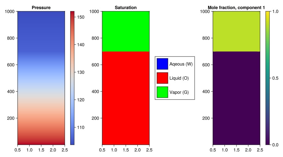
Set up a single-phase water model
We can also initialize single-phase models, which are entirely parametrized by the contact depth and pressure.
sys_1ph = SinglePhaseSystem(reference_density = 1000.0)
model_1ph = setup_reservoir_model(reservoir, sys_1ph)
eql_1ph = EquilibriumRegion(model_1ph, 100*bar, 1000.0)
state0_1ph = setup_reservoir_state(model_1ph, eql_1ph)
plot_state0(state0_1ph)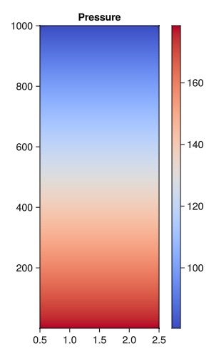
Set up two-phase water gas
A special case occurs for water-gas systems, where we have to specify the wgc instead of woc/goc. Otherwise, the equilibration is performed in much the same manner.
rhoS = [1000.0, 100.0]
sys_wg = ImmiscibleSystem((W, G), reference_densities = rhoS)
rho = ConstantCompressibilityDensities(sys_wg, 1.5bar, rhoS, 1e-5/bar)
model_wg = setup_reservoir_model(reservoir, sys_wg)
set_secondary_variables!(model_wg[:Reservoir], PhaseMassDensities = rho)

eql = EquilibriumRegion(model_wg, 100*bar, 1000.0, wgc = 1300.0)
state0_wg_eql = setup_reservoir_state(model_wg, eql)
plot_state0(state0_wg_eql, :wg)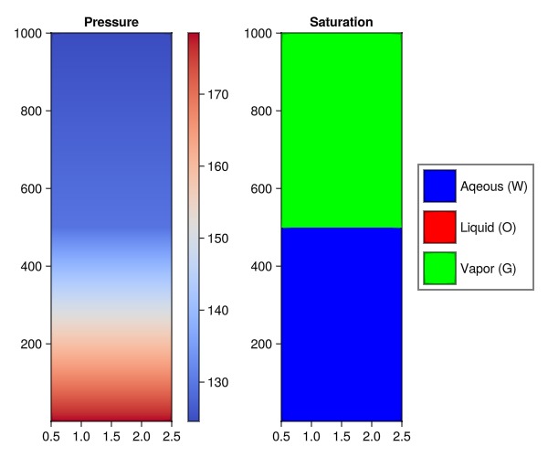
Conclusion
We have seen how to set up the initial state of a reservoir model using both direct assignment and hydrostatic equilibrium. Even a simple model can have surprising complexity in how the initial state should be set up. We have not covered all the options available (e.g. specifying capillary pressure interfaces), but the examples should give a good idea of how to set up your own model.
Example on GitHub
If you would like to run this example yourself, it can be downloaded from the JutulDarcy.jl GitHub repository as a script
This example took 37.059384151 seconds to complete.This page was generated using Literate.jl.