
Introduction to history matching with gradients
Immiscible HistoryMatching Introduction StartToFinish DifferentiabilityWe demonstrate the history matching functionality on a very simple 2D model. This example is intended to show the basic functionality in a self-contained script. History matching is a parameter estimation problem where we want to find the model parameters that minimize the mismatch against some observed data.
Model setup
We setup a 2D reservoir with a single injector and a single producer. This part of the example is conceptually similar to the Your first JutulDarcy.jl simulation and we do not go into detail on this part of the setup.
using JutulDarcy, Jutul
meter = si_unit(:meter)
kg = si_unit(:kg)
day = si_unit(:day)
bar = si_unit(:bar)
millidarcy = si_unit(:millidarcy)9.86923266716013e-16Mesh and system
nx = ny = 10
Lx = Ly = 100.0*meter
Lz = 10.0*meter
g = reservoir_mesh(nx = nx, ny = ny, nz = 1, Lx = Lx, Ly = Ly, Lz = Lz)
phases = (AqueousPhase(), LiquidPhase())
rhoAS = 1000.0kg/meter^3
rhoLS = 700.0kg/meter^3
reference_densities = [rhoAS, rhoLS]
sys = ImmiscibleSystem(phases, reference_densities = reference_densities)
ImmiscibleSystem with AqueousPhase, LiquidPhaseWell constraints and report steps
nstep = 25
dt = fill(365.0day, nstep)
inj_rate = 0.5*(Lx*Ly*Lz)/sum(dt)
I_ctrl = setup_injector_control(inj_rate, :rate, [1.0, 0.0], density = rhoAS)
P_ctrl = setup_producer_control(100bar, :bhp)
ProducerControl{BottomHolePressureTarget{Float64}, Float64}(BottomHolePressureTarget with value 100.0 [bar], 1.0)Build a parametrized simulation case
If we want to do history matching or optimize a model, we need to be able to systematically change the model based on our optimzation variables. In JutulDarcy, this is done by defining a function that takes a dictionary of parameters and returns a JutulCase object. This is a very powerful concept, as it affords the user complete freedom in how to define the model and how to map the optimization parameters to the model.
Define the truth case
We want to have a model where we can generate synthetic data to use for history matching. We define a dictionary of parameters that we will use to build the "truth" case. In this case, we will use the permeability, porosity and initial water saturation as our optimization parameters. These entries can also be vectors or matrices of numbers, but we will just use one number per parameter here.
prm_truth = Dict(
    "perm" => 100.0,
    "poro" => 0.2,
    "sw0" => 0.2
)
Dict{String, Float64} with 3 entries:
"perm" => 100.0
"sw0" => 0.2
"poro" => 0.2Define the function that builds the case
Now that we have decided on a dict format, we can make a function that takes a parameter dictionary and returns a JutulCase object (i.e. a complete model setup). We can reuse existing objects to avoid expensive resetup on each call during the optimization if the objects are not dependent on the optimization parameters.
Note the input arguments: The function takes a parameter dictionary and an optional dict that gives additional information about the current timestep being looked at by the optimizer, which is rarely used for history matching.
function build_case(prm::AbstractDict, step_info = missing)
    reservoir = reservoir_domain(g,
        permeability = prm["perm"]*millidarcy,
        porosity = prm["poro"]
    )
    I = setup_vertical_well(reservoir, 1, 1, name = :Injector)
    P = setup_well(reservoir, (nx, ny, 1), name = :Producer)
    model = setup_reservoir_model(reservoir, sys, wells = [I, P])

    sw0 = prm["sw0"]
    state0 = setup_reservoir_state(model,
        Pressure = 180*bar,
        Saturations = [sw0, 1-sw0]
    )
    controls = Dict(:Injector => I_ctrl, :Producer => P_ctrl)
    forces = setup_reservoir_forces(model, control = controls)
    return JutulCase(model, dt, forces, state0 = state0)
end
build_case (generic function with 2 methods)Verify that the case can be built and simulated
We set up an initial guess and verify that the function works by building the truth case and simulating it. This will also provide us with the data that we will use for history matching.
case_truth = build_case(prm_truth)
result_truth = simulate_reservoir(case_truth)
ReservoirSimResult with 25 entries:
wells (2 present):
:Producer
:Injector
Results per well:
:wrat => Vector{Float64} of size (25,)
:Aqueous_mass_rate => Vector{Float64} of size (25,)
:orat => Vector{Float64} of size (25,)
:bhp => Vector{Float64} of size (25,)
:mrat => Vector{Float64} of size (25,)
:lrat => Vector{Float64} of size (25,)
:mass_rate => Vector{Float64} of size (25,)
:rate => Vector{Float64} of size (25,)
:control => Vector{Symbol} of size (25,)
:Liquid_mass_rate => Vector{Float64} of size (25,)
:wcut => Vector{Float64} of size (25,)
states (Vector with 25 entries, reservoir variables for each state)
:Pressure => Vector{Float64} of size (100,)
:Saturations => Matrix{Float64} of size (2, 100)
:TotalMasses => Matrix{Float64} of size (2, 100)
time (report time for each state)
Vector{Float64} of length 25
result (extended states, reports)
SimResult with 25 entries
extra
Dict{Any, Any} with keys :simulator, :config
Completed at Oct. 09 2026 11:53 after 1 second, 818 milliseconds, 522.5 microseconds.History match the model
To be able to define an optimization problem we need four things:
A parametrized function that builds the model.
A set of parameters that we want to optimize with sensible absolute or relative bounds.
An objective function that takes the model and the simulation result and returns a scalar value that we want to minimize.
A starting point for the optimizer that is within the bounds.
### Define the initial guessWe define an initial guess for the optimization parameters. This is a dict with the same format as the truth case, but with different values.
prm_guess = Dict(
    "perm" => 50.0,
    "poro" => 0.15,
    "sw0" => 0.25
)
Dict{String, Float64} with 3 entries:
"perm" => 50.0
"sw0" => 0.25
"poro" => 0.15Set up the optimization problem
We can now set up the optimization problem. This will create an object that contains all the information about the optimization problem. We can then free parameters to be optimized and set bounds on them. We can also lump parameters and set scaling factors for each of the variables here.
opt = setup_reservoir_dict_optimization(prm_guess, build_case)
free_optimization_parameter!(opt, "perm", abs_min = 1.0, abs_max = 1000.0)
free_optimization_parameter!(opt, "poro", abs_min = 0.05, abs_max = 0.5)
free_optimization_parameter!(opt, "sw0", abs_min = 0.0, abs_max = 1.0)
DictParameters with 3 parameters (3 active), and 0 multipliers:
Active optimization parameters
┌──────┬───────────────┬───────┬──────┬────────┐
│ Name │ Initial value │ Count │ Min │ Max │
├──────┼───────────────┼───────┼──────┼────────┤
│ perm │ 50.0 │ 1 │ 1.0 │ 1000.0 │
│ poro │ 0.15 │ 1 │ 0.05 │ 0.5 │
│ sw0 │ 0.25 │ 1 │ 0.0 │ 1.0 │
└──────┴───────────────┴───────┴──────┴────────┘
No inactive optimization parameters.
No multipliers set.Load the history matching functionality
We can now load the history matching functionality and define an objective function that will be used to evaluate the mismatch between the model and the data. We could also have read (read_summary) or manually constructed a summary file to load data.
import JutulDarcy.HistoryMatching: history_match_objective, match_injectors!, match_producers!
obj = history_match_objective(case_truth, result_truth)
SumHistoryMatchObjective
HistoryMatch objective covering case with 24 years, 51 weeks, 2.18 days total simulation time
┌──────┬──────┬──────────┬────────┬───────┐
│ Well │ Type │ Quantity │ Weight │ Scale │
└──────┴──────┴──────────┴────────┴───────┘Define what values to match
We can now define what values we want to match. In this case, we will match the bottom hole pressure of the injector and water and oil rates of the producer. We can also set weights for the different objectives, which will be used to scale the contributions to the objective function. The weights can be one value per reporting timestep (case.dt) or a single value that will be used for all timesteps. Weights balance the importance of different wells and measurables. The default scaling of each type of well response is intended to scale the values to be around unit range for typical values, but this obviously depends on the specific model.
match_injectors!(obj, "WBHP", weight = 1.0)
match_producers!(obj, "WWPR", weight = 30.0)
match_producers!(obj, "WOPR", weight = 30.0)
HistoryMatch objective covering case with 24 years, 51 weeks, 2.18 days total simulation time
┌──────────┬──────────┬──────────┬────────┬─────────────┐
│ Well │ Type │ Quantity │ Weight │ Scale │
├──────────┼──────────┼──────────┼────────┼─────────────┤
│ Injector │ Injector │ WBHP │ 1.0 │ 1.15741e-11 │
│ Producer │ Producer │ WOPR │ 30.0 │ 0.00810185 │
│ Producer │ Producer │ WWPR │ 30.0 │ 0.0115741 │
└──────────┴──────────┴──────────┴────────┴─────────────┘Run the optimizer
We know how to set up a model, we know the bounds and we have defined an objective. We call the optimizer. For such a simple case, it will recover the parameters exactly in a few iterations. In general, the history match problem is ill-posed and the optimizer may not converge to a unique solution.
prm_opt = optimize_reservoir(opt, obj)
display(opt)
Optimization: Starting calibration of 3 parameters.
Jutul: Simulating 24 years, 51.31 weeks as 25 report steps
Optimization: Setting up adjoint storage.
Optimization: Finished setup in 38.666360562 seconds.
Optimization: Adjoint solve took 23.290849776 seconds.
Optimization: Objective #1: 1.33270e+07, gradient 2-norm: 2.74160e+08
It. | Objective | Proj. grad | Linesearch-its
-----------------------------------------------
0 | 4.8610e-02 | 1.6390e+00 | -
Jutul: Simulating 24 years, 51.31 weeks as 25 report steps
Optimization: Adjoint solve took 0.047301198 seconds.
Optimization: Objective #2: 6.13015e+06 (f/f0=4.600e-01), gradient 2-norm: 2.38333e+08
1 | 2.2360e-02 | 1.5698e+00 | 1
Jutul: Simulating 24 years, 51.31 weeks as 25 report steps
Optimization: Adjoint solve took 0.047653627 seconds.
Optimization: Objective #3: 4.53994e+06 (f/f0=3.407e-01), gradient 2-norm: 2.02484e+08
2 | 1.6559e-02 | 3.8589e-01 | 1
Jutul: Simulating 24 years, 51.31 weeks as 25 report steps
Optimization: Adjoint solve took 0.049246341 seconds.
Optimization: Objective #4: 3.17632e+05 (f/f0=2.383e-02), gradient 2-norm: 9.02232e+06
3 | 1.1586e-03 | 3.2738e-01 | 1
Jutul: Simulating 24 years, 51.31 weeks as 25 report steps
Optimization: Adjoint solve took 0.047920929 seconds.
Optimization: Objective #5: 2.91103e+05 (f/f0=2.184e-02), gradient 2-norm: 4.34176e+06
4 | 1.0618e-03 | 4.4303e-02 | 1
Jutul: Simulating 24 years, 51.31 weeks as 25 report steps
Optimization: Adjoint solve took 0.05064016 seconds.
Optimization: Objective #6: 1.82644e+05 (f/f0=1.370e-02), gradient 2-norm: 6.80582e+06
5 | 6.6620e-04 | 4.2144e-02 | 1
Jutul: Simulating 24 years, 51.31 weeks as 25 report steps
Optimization: Adjoint solve took 0.046762237 seconds.
Optimization: Objective #7: 1.74222e+05 (f/f0=1.307e-02), gradient 2-norm: 5.77498e+05
6 | 6.3547e-04 | 1.2385e-02 | 1
Jutul: Simulating 24 years, 51.31 weeks as 25 report steps
Optimization: Adjoint solve took 0.048185907 seconds.
Optimization: Objective #8: 1.72543e+05 (f/f0=1.295e-02), gradient 2-norm: 2.00449e+05
7 | 6.2935e-04 | 6.6638e-03 | 1
Jutul: Simulating 24 years, 51.31 weeks as 25 report steps
Optimization: Adjoint solve took 0.048922212 seconds.
Optimization: Objective #9: 1.72506e+05 (f/f0=1.294e-02), gradient 2-norm: 7.98294e+04
8 | 6.2922e-04 | 8.4741e-04 | 1
Optimization: Finished in 68.646108907 seconds.Plot the results
This section requires plotting to be available.
using GLMakiePlot the base case
We can now plot the results of the history matching. We first do a plot to verify that the base case has zero objective.
import JutulDarcy: plot_mismatch
result_truth = simulate_reservoir(build_case(prm_truth))
plot_mismatch(obj, result_truth)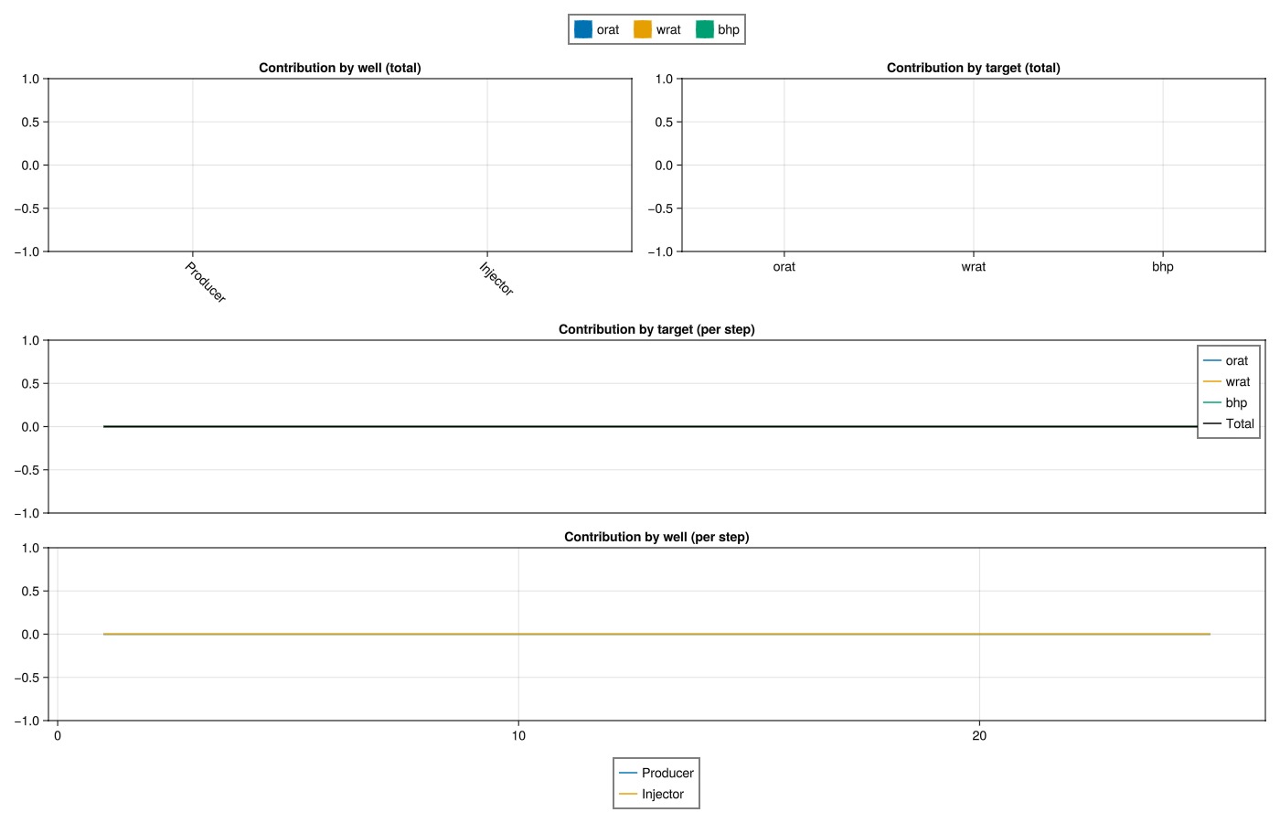
Plot the initial guess
result_guess = simulate_reservoir(build_case(prm_guess))
plot_mismatch(obj, result_guess)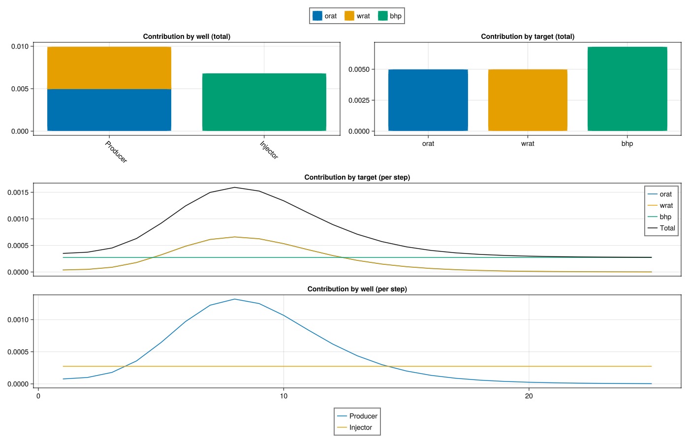
Plot the tuned case
We see that contributions to the objective function are now very small, indicating that the history matching has been successful.
result_tuned = simulate_reservoir(build_case(prm_opt))
plot_mismatch(obj, result_tuned)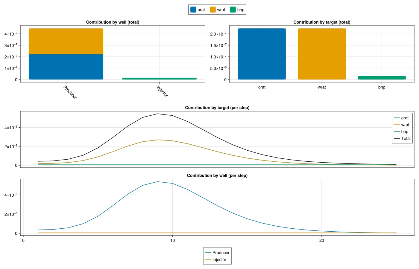
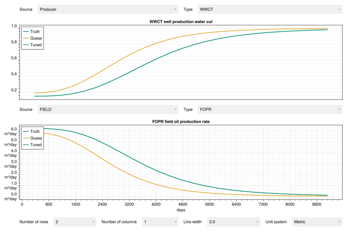
Plot the well responses
We see that we have successfully matched this model.
plot_summary(
    [result_truth, result_guess, result_tuned],
    names = ["Truth", "Guess", "Tuned"],
    plots = ["Producer:WWCT", "FOPR"]
)
Example on GitHub
If you would like to run this example yourself, it can be downloaded from the JutulDarcy.jl GitHub repository as a script
This example took 85.530233534 seconds to complete.This page was generated using Literate.jl.