Your first JutulDarcy.jl simulation
After a bit of time has passed compiling the packages, you are now ready to use JutulDarcy. There are a number of examples included in this manual, but we include a brief example here that briefly demonstrates the key concepts.
Setting up the domain
We set up a simple Cartesian Mesh that is converted into a reservoir domain with static properties permeability and porosity values together with geometry information. We then use this domain to set up two wells: One vertical well for injection and a single perforation producer.
using JutulDarcy, Jutul
Darcy, bar, kg, meter, day = si_units(:darcy, :bar, :kilogram, :meter, :day)
nx = ny = 25
nz = 10
cart_dims = (nx, ny, nz)
physical_dims = (1000.0, 1000.0, 100.0).*meter
g = CartesianMesh(cart_dims, physical_dims)
domain = reservoir_domain(g, permeability = 0.3Darcy, porosity = 0.2)
Injector = setup_vertical_well(domain, 1, 1, name = :Injector)
Producer = setup_well(domain, (nx, ny, 1), name = :Producer)
# Show the properties in the domain
domain
DataDomain wrapping CartesianMesh (3D) with 25x25x10=6250 cells with 17 data fields added:
6250 Cells
:permeability => 6250 Vector{Float64}
:porosity => 6250 Vector{Float64}
:rock_thermal_conductivity => 6250 Vector{Float64}
:fluid_thermal_conductivity => 6250 Vector{Float64}
:rock_density => 6250 Vector{Float64}
:cell_centroids => 3×6250 Matrix{Float64}
:volumes => 6250 Vector{Float64}
17625 Faces
:neighbors => 2×17625 Matrix{Int64}
:areas => 17625 Vector{Float64}
:normals => 3×17625 Matrix{Float64}
:face_centroids => 3×17625 Matrix{Float64}
35250 HalfFaces
:half_face_cells => 35250 Vector{Int64}
:half_face_faces => 35250 Vector{Int64}
2250 BoundaryFaces
:boundary_areas => 2250 Vector{Float64}
:boundary_centroids => 3×2250 Matrix{Float64}
:boundary_normals => 3×2250 Matrix{Float64}
:boundary_neighbors => 2250 Vector{Int64}Setting up a fluid system
We select a two-phase immicible system by declaring that the liquid and vapor phases are present in the model. These are assumed to have densities of 1000 and 100 kilograms per meters cubed at reference pressure and temperature conditions.
phases = (LiquidPhase(), VaporPhase())
rhoLS = 1000.0kg/meter^3
rhoGS = 100.0kg/meter^3
reference_densities = [rhoLS, rhoGS]
sys = ImmiscibleSystem(phases, reference_densities = reference_densities)ImmiscibleSystem with LiquidPhase, VaporPhaseSetting up the model
We now have everything we need to set up a model. We call the reservoir model setup function and get out the model together with the parameters. Parameter represent numerical input values that are static throughout the simulation. These are automatically computed from the domain's geometry, permeability and porosity.
model, parameters = setup_reservoir_model(domain, sys, wells = [Injector, Producer])
modelMultiModel with 4 models and 6 cross-terms. 12539 equations, 12539 degrees of freedom and 54061 parameters.
models:
1) Reservoir (12500x12500)
ImmiscibleSystem with LiquidPhase, VaporPhase
∈ MinimalTPFATopology (6250 cells, 17625 faces)
2) Injector (32x32)
ImmiscibleSystem with LiquidPhase, VaporPhase
∈ MultiSegmentWell [Injector] (11 nodes, 10 segments, 10 perforations)
3) Producer (5x5)
ImmiscibleSystem with LiquidPhase, VaporPhase
∈ MultiSegmentWell [Producer] (2 nodes, 1 segments, 1 perforations)
4) Facility (2x2)
JutulDarcy.PredictionMode()
∈ WellGroup([:Injector, :Producer], true, true)
cross_terms:
1) Injector <-> Reservoir (Eq: mass_conservation)
JutulDarcy.ReservoirFromWellFlowCT
2) Producer <-> Reservoir (Eq: mass_conservation)
JutulDarcy.ReservoirFromWellFlowCT
3) Injector -> Facility (Eq: control_equation)
JutulDarcy.FacilityFromWellFlowCT
4) Facility -> Injector (Eq: mass_conservation)
JutulDarcy.WellFromFacilityFlowCT
5) Producer -> Facility (Eq: control_equation)
JutulDarcy.FacilityFromWellFlowCT
6) Facility -> Producer (Eq: mass_conservation)
JutulDarcy.WellFromFacilityFlowCT
Model storage will be optimized for runtime performance.The model has a set of default secondary variables (properties) that are used to compute the flow equations. We can have a look at the reservoir model to see what the defaults are for the Darcy flow part of the domain:
reservoir_model(model)SimulationModel:
Model with 12500 degrees of freedom, 12500 equations and 54000 parameters
domain:
DiscretizedDomain with MinimalTPFATopology (6250 cells, 17625 faces) and discretizations for mass_flow, heat_flow
system:
ImmiscibleSystem with LiquidPhase, VaporPhase
context:
DefaultContext(BlockMajorLayout(false), 1000, 1)
formulation:
FullyImplicitFormulation()
data_domain:
DataDomain wrapping CartesianMesh (3D) with 25x25x10=6250 cells with 17 data fields added:
  6250 Cells
    :permeability => 6250 Vector{Float64}
    :porosity => 6250 Vector{Float64}
    :rock_thermal_conductivity => 6250 Vector{Float64}
    :fluid_thermal_conductivity => 6250 Vector{Float64}
    :rock_density => 6250 Vector{Float64}
    :cell_centroids => 3×6250 Matrix{Float64}
    :volumes => 6250 Vector{Float64}
  17625 Faces
    :neighbors => 2×17625 Matrix{Int64}
    :areas => 17625 Vector{Float64}
    :normals => 3×17625 Matrix{Float64}
    :face_centroids => 3×17625 Matrix{Float64}
  35250 HalfFaces
    :half_face_cells => 35250 Vector{Int64}
    :half_face_faces => 35250 Vector{Int64}
  2250 BoundaryFaces
    :boundary_areas => 2250 Vector{Float64}
    :boundary_centroids => 3×2250 Matrix{Float64}
    :boundary_normals => 3×2250 Matrix{Float64}
    :boundary_neighbors => 2250 Vector{Int64}
primary_variables:
1) Pressure ∈ 6250 Cells: 1 dof each
2) Saturations ∈ 6250 Cells: 1 dof, 2 values each
secondary_variables:
1) PhaseMassDensities ∈ 6250 Cells: 2 values each
-> ConstantCompressibilityDensities as evaluator
2) TotalMasses ∈ 6250 Cells: 2 values each
-> TotalMasses as evaluator
3) RelativePermeabilities ∈ 6250 Cells: 2 values each
-> BrooksCoreyRelativePermeabilities as evaluator
4) PhaseMobilities ∈ 6250 Cells: 2 values each
-> JutulDarcy.PhaseMobilities as evaluator
5) PhaseMassMobilities ∈ 6250 Cells: 2 values each
-> JutulDarcy.PhaseMassMobilities as evaluator
parameters:
1) Transmissibilities ∈ 17625 Faces: Scalar
2) TwoPointGravityDifference ∈ 17625 Faces: Scalar
3) PhaseViscosities ∈ 6250 Cells: 2 values each
4) FluidVolume ∈ 6250 Cells: Scalar
equations:
1) mass_conservation ∈ 6250 Cells: 2 values each
-> ConservationLaw{:TotalMasses, TwoPointPotentialFlowHardCoded{Vector{Int64}, Vector{@NamedTuple{self::Int64, other::Int64, face::Int64, face_sign::Int64}}}, Jutul.DefaultFlux, 2}
output_variables:
Pressure, Saturations, TotalMasses
extra:
OrderedCollections.OrderedDict{Symbol, Any} with keys: Symbol[]The secondary variables can be swapped out, replaced and new variables can be added with arbitrary functional dependencies thanks to Jutul's flexible setup for automatic differentiation. Let us adjust the defaults by replacing the relative permeabilities with Brooks-Corey functions and the phase density functions by constant compressibilities:
c = [1e-6, 1e-4]/bar
density = ConstantCompressibilityDensities(
    p_ref = 100*bar,
    density_ref = reference_densities,
    compressibility = c
)
kr = BrooksCoreyRelativePermeabilities(sys, [2.0, 3.0])
replace_variables!(model, PhaseMassDensities = density, RelativePermeabilities = kr)
Initial state: Pressure and saturations
Now that we are happy with our model setup, we can designate an initial state. Equilibriation of reservoirs can be a complicated affair, but here we set up a constant pressure reservoir filled with the liquid phase. The inputs must match the primary variables of the model, which in this case is pressure and saturations in every cell.
state0 = setup_reservoir_state(model,
    Pressure = 120bar,
    Saturations = [1.0, 0.0]
)
Dict{Any, Any} with 4 entries:
:Producer => Dict{Symbol, Any}(:TotalMassFlux=>[0.0], :PhaseMassDensities=>[…
:Injector => Dict{Symbol, Any}(:TotalMassFlux=>[0.0, 0.0, 0.0, 0.0, 0.0, 0.0…
:Reservoir => Dict{Symbol, Any}(:PhaseMassMobilities=>[0.0 0.0 … 0.0 0.0; 0.0…
:Facility => Dict{Symbol, Any}(:TotalSurfaceMassRate=>[0.0, 0.0], :WellGroup…Setting up timesteps and well controls
We set up reporting timesteps. These are the intervals that the simulator gives out outputs. The simulator may use shorter steps internally, but will always hit these points in the output. Here, we report every year for 25 years.
nstep = 25
dt = fill(365.0day, nstep);
25-element Vector{Float64}:
3.1536e7
3.1536e7
3.1536e7
3.1536e7
3.1536e7
3.1536e7
3.1536e7
3.1536e7
3.1536e7
3.1536e7
⋮
3.1536e7
3.1536e7
3.1536e7
3.1536e7
3.1536e7
3.1536e7
3.1536e7
3.1536e7
3.1536e7We next set up a rate target with a high amount of gas injected into the model. This is not fully realistic, but will give some nice and dramatic plots for our example later on.
pv = pore_volume(model, parameters)
inj_rate = 1.5*sum(pv)/sum(dt)
rate_target = TotalRateTarget(inj_rate)
TotalRateTarget with value 0.0380517503805175 [m^3/s]The producer is set to operate at a fixed pressure:
bhp_target = BottomHolePressureTarget(100bar)BottomHolePressureTarget with value 100.0 [bar]We can finally set up forces for the model. Note that while JutulDarcy supports time-dependent forces and limits for the wells, we keep this example as simple as possible.
I_ctrl = InjectorControl(rate_target, [0.0, 1.0], density = rhoGS)
P_ctrl = ProducerControl(bhp_target)
controls = Dict(:Injector => I_ctrl, :Producer => P_ctrl)
forces = setup_reservoir_forces(model, control = controls);
Dict{Symbol, Any} with 4 entries:
:Producer => (mask = nothing,)
:Injector => (mask = nothing,)
:Reservoir => (bc = nothing, sources = nothing)
:Facility => (control = Dict{Symbol, WellControlForce}(:Producer=>ProducerCo…Simulate and analyze results
We call the simulation with our initial state, our model, the timesteps, the forces and the parameters:
wd, states, t = simulate_reservoir(state0, model, dt, parameters = parameters, forces = forces)ReservoirSimResult with 25 entries:
wells (2 present):
:Producer
:Injector
Results per well:
:Vapor_mass_rate => Vector{Float64} of size (25,)
:lrat => Vector{Float64} of size (25,)
:orat => Vector{Float64} of size (25,)
:control => Vector{Symbol} of size (25,)
:bhp => Vector{Float64} of size (25,)
:Liquid_mass_rate => Vector{Float64} of size (25,)
:mass_rate => Vector{Float64} of size (25,)
:rate => Vector{Float64} of size (25,)
:grat => Vector{Float64} of size (25,)
states (Vector with 25 entries, reservoir variables for each state)
:Saturations => Matrix{Float64} of size (2, 6250)
:Pressure => Vector{Float64} of size (6250,)
:TotalMasses => Matrix{Float64} of size (2, 6250)
time (report time for each state)
Vector{Float64} of length 25
result (extended states, reports)
SimResult with 25 entries
extra
Dict{Any, Any} with keys :simulator, :config
Completed at Oct. 01 2024 16:10 after 5 seconds, 91 milliseconds, 616.6 microseconds.We can interactively look at the well results in the command line:
wd(:Producer)Legend
┌──────────────────┬──────────────────────────────────────────┬──────┬─────────────────────────┐
│ Label │ Description │ Unit │ Type of quantity │
├──────────────────┼──────────────────────────────────────────┼──────┼─────────────────────────┤
│ Liquid_mass_rate │ Component mass rate for Liquid component │ kg/s │ mass │
│ Vapor_mass_rate │ Component mass rate for Vapor component │ kg/s │ mass │
│ bhp │ Bottom hole pressure │ Pa │ pressure │
│ control │ Control │ - │ none │
│ grat │ Surface gas rate │ m³/s │ surface_volume_per_time │
│ lrat │ Surface water rate │ m³/s │ surface_volume_per_time │
│ mass_rate │ Total mass rate │ kg/s │ mass │
│ orat │ Surface oil rate │ m³/s │ surface_volume_per_time │
│ rate │ Surface total rate │ m³/s │ surface_volume_per_time │
└──────────────────┴──────────────────────────────────────────┴──────┴─────────────────────────┘
Producer result
┌────────┬──────────────────┬─────────────────┬───────┬─────────┬─────────────┬─────────────┬───────────┬─────────────┬────────────┐
│ time │ Liquid_mass_rate │ Vapor_mass_rate │ bhp │ control │ grat │ lrat │ mass_rate │ orat │ rate │
│ days │ kg/s │ kg/s │ Pa │ - │ m³/s │ m³/s │ kg/s │ m³/s │ m³/s │
├────────┼──────────────────┼─────────────────┼───────┼─────────┼─────────────┼─────────────┼───────────┼─────────────┼────────────┤
│ 365.0 │ -37.5272 │ -0.0 │ 1.0e7 │ bhp │ -0.0 │ -0.0375272 │ -37.5272 │ -0.0375272 │ -0.0375272 │
│ 730.0 │ -37.5372 │ -0.0 │ 1.0e7 │ bhp │ -0.0 │ -0.0375372 │ -37.5372 │ -0.0375372 │ -0.0375372 │
│ 1095.0 │ -37.5455 │ -0.0 │ 1.0e7 │ bhp │ -0.0 │ -0.0375455 │ -37.5455 │ -0.0375455 │ -0.0375455 │
│ 1460.0 │ -37.5474 │ -0.0 │ 1.0e7 │ bhp │ -0.0 │ -0.0375474 │ -37.5474 │ -0.0375474 │ -0.0375474 │
│ 1825.0 │ -37.5515 │ -0.0 │ 1.0e7 │ bhp │ -0.0 │ -0.0375515 │ -37.5515 │ -0.0375515 │ -0.0375515 │
│ 2190.0 │ -37.5532 │ -0.0 │ 1.0e7 │ bhp │ -0.0 │ -0.0375532 │ -37.5532 │ -0.0375532 │ -0.0375532 │
│ 2555.0 │ -37.5505 │ -0.0 │ 1.0e7 │ bhp │ -0.0 │ -0.0375505 │ -37.5505 │ -0.0375505 │ -0.0375505 │
│ 2920.0 │ -33.8661 │ -0.109282 │ 1.0e7 │ bhp │ -0.00109282 │ -0.0338661 │ -33.9754 │ -0.0338661 │ -0.0349589 │
│ 3285.0 │ -32.0501 │ -0.425517 │ 1.0e7 │ bhp │ -0.00425517 │ -0.0320501 │ -32.4756 │ -0.0320501 │ -0.0363052 │
│ 3650.0 │ -29.0912 │ -0.734914 │ 1.0e7 │ bhp │ -0.00734914 │ -0.0290912 │ -29.8262 │ -0.0290912 │ -0.0364404 │
│ 4015.0 │ -26.3369 │ -1.04161 │ 1.0e7 │ bhp │ -0.0104161 │ -0.0263369 │ -27.3785 │ -0.0263369 │ -0.036753 │
│ 4380.0 │ -23.8608 │ -1.31842 │ 1.0e7 │ bhp │ -0.0131842 │ -0.0238608 │ -25.1792 │ -0.0238608 │ -0.037045 │
│ 4745.0 │ -21.4534 │ -1.57833 │ 1.0e7 │ bhp │ -0.0157833 │ -0.0214534 │ -23.0317 │ -0.0214534 │ -0.0372367 │
│ 5110.0 │ -19.4122 │ -1.80125 │ 1.0e7 │ bhp │ -0.0180125 │ -0.0194122 │ -21.2135 │ -0.0194122 │ -0.0374247 │
│ 5475.0 │ -17.4981 │ -2.00816 │ 1.0e7 │ bhp │ -0.0200816 │ -0.0174981 │ -19.5063 │ -0.0174981 │ -0.0375797 │
│ 5840.0 │ -15.8785 │ -2.18061 │ 1.0e7 │ bhp │ -0.0218061 │ -0.0158785 │ -18.0591 │ -0.0158785 │ -0.0376846 │
│ 6205.0 │ -14.2389 │ -2.35803 │ 1.0e7 │ bhp │ -0.0235803 │ -0.0142389 │ -16.597 │ -0.0142389 │ -0.0378192 │
│ 6570.0 │ -12.9669 │ -2.49084 │ 1.0e7 │ bhp │ -0.0249084 │ -0.0129669 │ -15.4578 │ -0.0129669 │ -0.0378753 │
│ 6935.0 │ -11.728 │ -2.62309 │ 1.0e7 │ bhp │ -0.0262309 │ -0.011728 │ -14.3511 │ -0.011728 │ -0.0379589 │
│ 7300.0 │ -10.4742 │ -2.75799 │ 1.0e7 │ bhp │ -0.0275799 │ -0.0104742 │ -13.2322 │ -0.0104742 │ -0.0380541 │
│ 7665.0 │ -9.50529 │ -2.85645 │ 1.0e7 │ bhp │ -0.0285645 │ -0.00950529 │ -12.3617 │ -0.00950529 │ -0.0380697 │
│ 8030.0 │ -8.6432 │ -2.94597 │ 1.0e7 │ bhp │ -0.0294597 │ -0.0086432 │ -11.5892 │ -0.0086432 │ -0.0381029 │
│ 8395.0 │ -7.70208 │ -3.04928 │ 1.0e7 │ bhp │ -0.0304928 │ -0.00770208 │ -10.7514 │ -0.00770208 │ -0.0381948 │
│ 8760.0 │ -6.81005 │ -3.1436 │ 1.0e7 │ bhp │ -0.031436 │ -0.00681005 │ -9.95365 │ -0.00681005 │ -0.038246 │
│ 9125.0 │ -6.12761 │ -3.20964 │ 1.0e7 │ bhp │ -0.0320964 │ -0.00612761 │ -9.33725 │ -0.00612761 │ -0.038224 │
└────────┴──────────────────┴─────────────────┴───────┴─────────┴─────────────┴─────────────┴───────────┴─────────────┴────────────┘Let us look at the pressure evolution in the injector:
wd(:Injector, :bhp)Legend
┌───────┬──────────────────────┬──────┬──────────────────┐
│ Label │ Description │ Unit │ Type of quantity │
├───────┼──────────────────────┼──────┼──────────────────┤
│ bhp │ Bottom hole pressure │ Pa │ pressure │
└───────┴──────────────────────┴──────┴──────────────────┘
Injector result
┌────────┬───────────┐
│ time │ bhp │
│ days │ Pa │
├────────┼───────────┤
│ 365.0 │ 2.74397e7 │
│ 730.0 │ 2.71983e7 │
│ 1095.0 │ 2.7083e7 │
│ 1460.0 │ 2.70379e7 │
│ 1825.0 │ 2.70048e7 │
│ 2190.0 │ 2.69884e7 │
│ 2555.0 │ 2.69939e7 │
│ 2920.0 │ 3.27559e7 │
│ 3285.0 │ 3.7432e7 │
│ 3650.0 │ 3.99756e7 │
│ 4015.0 │ 4.15342e7 │
│ 4380.0 │ 4.24638e7 │
│ 4745.0 │ 4.29401e7 │
│ 5110.0 │ 4.3123e7 │
│ 5475.0 │ 4.30622e7 │
│ 5840.0 │ 4.28891e7 │
│ 6205.0 │ 4.25667e7 │
│ 6570.0 │ 4.21921e7 │
│ 6935.0 │ 4.17739e7 │
│ 7300.0 │ 4.1256e7 │
│ 7665.0 │ 4.07498e7 │
│ 8030.0 │ 4.02601e7 │
│ 8395.0 │ 3.96922e7 │
│ 8760.0 │ 3.90606e7 │
│ 9125.0 │ 3.84919e7 │
└────────┴───────────┘If we have a plotting package available, we can visualize the results too:
using GLMakie
grat = wd[:Producer, :grat]
lrat = wd[:Producer, :lrat]
bhp = wd[:Injector, :bhp]
fig = Figure(size = (1200, 400))
ax = Axis(fig[1, 1],
    title = "Injector",
    xlabel = "Time / days",
    ylabel = "Bottom hole pressure / bar")
lines!(ax, t/day, bhp./bar)
ax = Axis(fig[1, 2],
    title = "Producer",
    xlabel = "Time / days",
    ylabel = "Production rate / m³/day")
lines!(ax, t/day, abs.(grat).*day)
lines!(ax, t/day, abs.(lrat).*day)
fig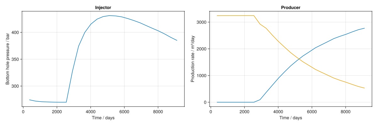
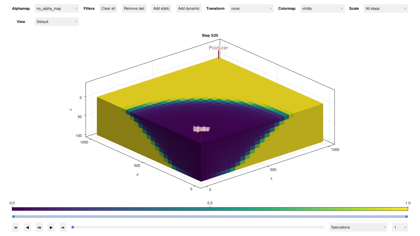
Interactive visualization of the 3D results is also possible if GLMakie is loaded:
plot_reservoir(model, states, key = :Saturations, step = 3)