Simulating Eclipse/DATA input files
The DATA format is commonly used in reservoir simulation. JutulDarcy can set up cases on this format and includes a fully featured grid builder for corner-point grids. Once a case has been set up, it uses the same types as a regular JutulDarcy simulation, allowing modification and use of the case in differentiable workflows.
We begin by loading the SPE9 dataset via the GeoEnergyIO package.
using JutulDarcy
pth = JutulDarcy.GeoEnergyIO.test_input_file_path("SPE9", "SPE9.DATA")"/home/runner/.julia/artifacts/c1063fdc96b21cbc18ea8a3bd1a1281aa04ffa3f/SPE9.DATA"Set up and run a simulation
If we do not need the case, we could also have done: ws, states = simulate_data_file(pth)
case = setup_case_from_data_file(pth)
ws, states = simulate_reservoir(case)
ReservoirSimResult with 90 entries:
wells (26 present):
:INJE1
:PRODU25
:PRODU16
:PRODU20
:PRODU10
:PRODU12
:PRODU22
:PRODU14
:PRODU6
:PRODU7
:PRODU9
:PRODU24
:PRODU3
:PRODU23
:PRODU5
:PRODU11
:PRODU17
:PRODU4
:PRODU15
:PRODU2
:PRODU19
:PRODU21
:PRODU13
:PRODU8
:PRODU26
:PRODU18
Results per well:
:wrat => Vector{Float64} of size (90,)
:Aqueous_mass_rate => Vector{Float64} of size (90,)
:orat => Vector{Float64} of size (90,)
:bhp => Vector{Float64} of size (90,)
:lrat => Vector{Float64} of size (90,)
:mass_rate => Vector{Float64} of size (90,)
:rate => Vector{Float64} of size (90,)
:Vapor_mass_rate => Vector{Float64} of size (90,)
:control => Vector{Symbol} of size (90,)
:Liquid_mass_rate => Vector{Float64} of size (90,)
:grat => Vector{Float64} of size (90,)
states (Vector with 90 entries, reservoir variables for each state)
:BlackOilUnknown => Vector{BlackOilX{Float64}} of size (9000,)
:Saturations => Matrix{Float64} of size (3, 9000)
:Pressure => Vector{Float64} of size (9000,)
:Rs => Vector{Float64} of size (9000,)
:ImmiscibleSaturation => Vector{Float64} of size (9000,)
:TotalMasses => Matrix{Float64} of size (3, 9000)
time (report time for each state)
Vector{Float64} of length 90
result (extended states, reports)
SimResult with 90 entries
extra
Dict{Any, Any} with keys :simulator, :config
Completed at Oct. 01 2024 16:10 after 12 seconds, 682 milliseconds, 385.2 microseconds.Show the input data
The input data takes the form of a Dict:
case.input_dataDict{String, Any} with 6 entries:
"RUNSPEC" => OrderedDict{String, Any}("TITLE"=>"SPE 9", "DIMENS"=>[24, 25, 1…
"GRID" => OrderedDict{String, Any}("cartDims"=>(24, 25, 15), "CURRENT_BOX…
"PROPS" => OrderedDict{String, Any}("PVTW"=>Any[[2.48211e7, 1.0034, 4.3511…
"SUMMARY" => OrderedDict{String, Any}()
"SCHEDULE" => Dict{String, Any}("STEPS"=>OrderedDict{String, Any}[OrderedDict…
"SOLUTION" => OrderedDict{String, Any}("EQUIL"=>Any[[2753.87, 2.48211e7, 3032…We can also examine the RUNSPEC section
case.input_data["RUNSPEC"]OrderedCollections.OrderedDict{String, Any} with 13 entries:
"TITLE" => "SPE 9"
"DIMENS" => [24, 25, 15]
"OIL" => true
"WATER" => true
"GAS" => true
"DISGAS" => true
"FIELD" => true
"START" => DateTime("2015-01-01T00:00:00")
"WELLDIMS" => [26, 5, 1, 26, 5, 10, 5, 4, 3, 0, 1, 1, 10, 201]
"TABDIMS" => [1, 1, 40, 20, 1, 20, 20, 1, 1, -1 … -1, 10, 10, 10, -1, 5, 5…
"EQLDIMS" => [1, 100, 50, 1, 50]
"UNIFIN" => true
"UNIFOUT" => truePlot the simulation model
These plot are interactive when run outside of the documentations.
using GLMakie
plot_reservoir(case.model, states)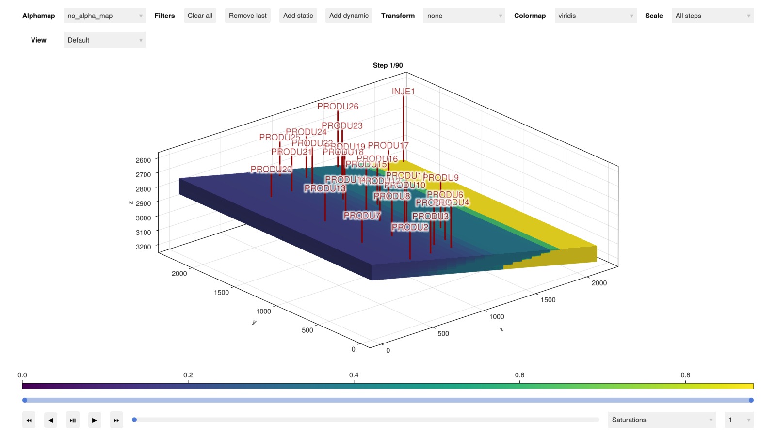
Plot the well responses
plot_well_results(ws)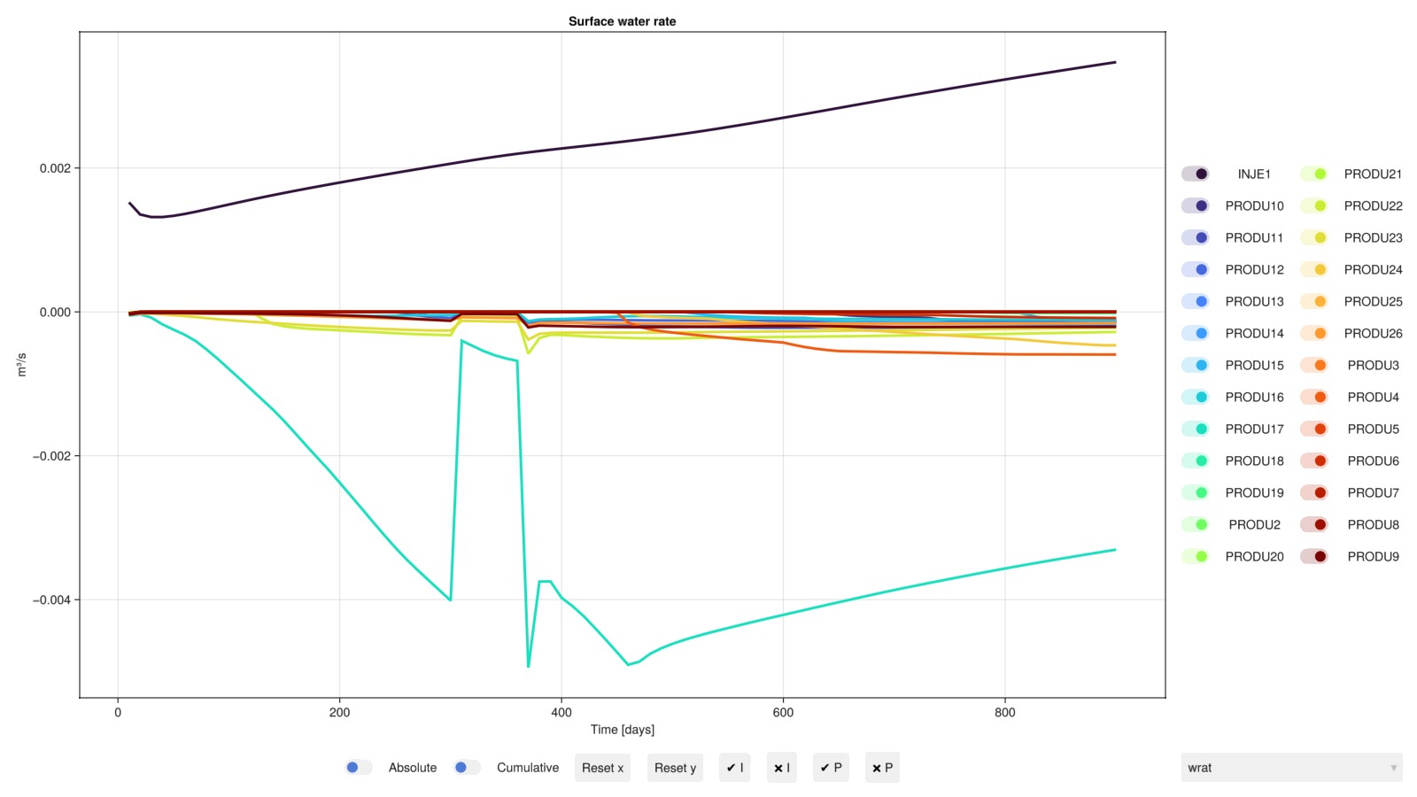
Example on GitHub
If you would like to run this example yourself, it can be downloaded from the JutulDarcy.jl GitHub repository as a script, or as a Jupyter Notebook
This page was generated using Literate.jl.