Validation of equation-of-state compositional simulator

This example solves a 1D two-phase, three component miscible displacement problem and compares against existing simulators (E300, AD-GPRS) to verify correctness.

The case is loaded from an input file that can be run in other simulators. For convenience, we provide solutions from the other simulators as a binary file to perform a comparison without having to run and convert results from other the simulators.

This case is a small compositional problem inspired by the examples in Voskov et al (JPSE, 2012). A 1D reservoir of 1,000 meters length is discretized into 1,000 cells. The model initially contains a mixture made up of 0.6 parts C10, 0.1 parts CO2, and 0.3 parts C1 by moles at 150 degrees C and 75 bar pressure. Wells are placed in the leftmost and rightmost cells of the domain, with the leftmost well injecting pure CO $_{2}$ at a fixed bottom-hole pressure of 100 bar and the other well producing at 50 bar. The model is isothermal and contains a phase transition from the initial two-phase mixture to single-phase gas as injected CO $_{2}$ eventually displaces the resident fluids. For further details on this setup, see Møyner and Tchelepi (SPE J. 2018) [8].

julia

using JutulDarcy
using Jutul
using GLMakie
dpth = JutulDarcy.GeoEnergyIO.test_input_file_path("SIMPLE_COMP")
data_path = joinpath(dpth, "SIMPLE_COMP.DATA")
case = setup_case_from_data_file(data_path)
result = simulate_reservoir(case, info_level = -1)
ws, states = result;

Plot solutions and compare

The 1D displacement can be plotted as a line plot. We pick a step midway through the simulation and plot compositions, saturations and pressure.

julia

cmap = :tableau_hue_circle
ref_path = joinpath(dpth, "reference.jld2")
ref = Jutul.JLD2.load(ref_path)

step_to_plot = 250
fig = with_theme(theme_latexfonts()) do
    x = reservoir_domain(case)[:cell_centroids][1, :]
    mz = 3
    ix = step_to_plot
    mt = :circle
    fig = Figure(size = (800, 400))
    ax = Axis(fig[2, 1], xlabel = "Cell center / m")
    cnames = ["DECANE", "CO2", "METHANE"]
    cnames = ["C₁₀", "CO₂", "C₁"]
    cnames = [L"\text{C}_{10}", L"\text{CO}_2", L"\text{C}_1"]
    lineh = []
    lnames = []
    crange = (1, 4)
    for i in range(crange...)
        if i == 4
            cname = L"\text{S}_g"
            gprs = missing
            ecl = ref["e300"][ix][:Saturations][2, :]
            ju = states[ix][:Saturations][2, :]
        else
            @assert i <= 4
            ecl = ref["e300"][ix][:OverallMoleFractions][i, :]
            gprs = ref["adgprs"][ix][:OverallMoleFractions][i, :]
            ju = states[ix][:OverallMoleFractions][i, :]
            cname = cnames[i]
        end
        h = lines!(ax, x, ju, colormap = cmap, color = i, colorrange = crange, label = cname)
        push!(lnames, cname)
        push!(lineh, h)
        scatter!(ax, x, ecl, markersize = mz, colormap = cmap, color = i, colorrange = crange)
        if !ismissing(gprs)
            lines!(ax, x, gprs, colormap = cmap, color = i, colorrange = crange, linestyle = :dash)
        end
    end

    l_ju = LineElement(color = :black, linestyle = nothing)
    l_ecl = MarkerElement(color = :black, markersize = mz, marker = mt)
    l_gprs = LineElement(color = :black, linestyle = :dash)

    Legend(
        fig[1, 1],
        [[l_ju, l_ecl, l_gprs], lineh],
        [[L"\text{JutulDarcy}", L"\text{E300}", L"\text{AD-GPRS}"], lnames],
        ["Simulator", "Result"],
        tellwidth = false,
        orientation = :horizontal,
    )
    fig
end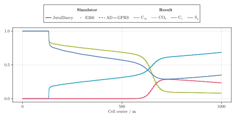

Calculate sensitivities

We demonstrate how the parameter sensitivities of an objective function can be calculated for a compositional model.

The objective function is taken to be the average gas saturation at a specific report step that was plotted in the previous section.

julia

import Statistics: mean
import JutulDarcy: reservoir_sensitivities
function objective_function(model, state, Δt, step_i, forces)
    if step_i != step_to_plot
        return 0.0
    end
    sg = @view state.Reservoir.Saturations[2, :]
    return mean(sg)
end
data_domain_with_gradients = reservoir_sensitivities(case, result, objective_function, include_parameters = true)

fig = with_theme(theme_latexfonts()) do
    x = reservoir_domain(case)[:cell_centroids][1, :]
    mz = 3
    ix = step_to_plot
    cmap = :Dark2_5
    cmap = :Accent_4
    cmap = :Spectral_4
    cmap = :tableau_hue_circle
    mt = :circle
    fig = Figure(size = (800, 400))
    normalize = x -> x./(maximum(x) - minimum(x))
    logscale = x -> sign.(x).*log10.(abs.(x))

    ∂T = data_domain_with_gradients[:temperature]
    ∂ϕ = data_domain_with_gradients[:porosity]

    ax1 = Axis(fig[2, 1], yticklabelcolor = :blue, xlabel = "Cell center / m")
    ax2 = Axis(fig[2, 1], yticklabelcolor = :red, yaxisposition = :right)
    hidespines!(ax2)
    hidexdecorations!(ax2)

    l1 = lines!(ax1, x, ∂T, label = "Temperature", color = :blue)
    l2 = lines!(ax2, x, ∂ϕ, label = "Porosity", color = :red)

    Legend(fig[1, 1], [l1, l2], ["Temperature", "Porosity"], "Parameter", tellwidth = false, orientation = :horizontal)
    fig
end
fig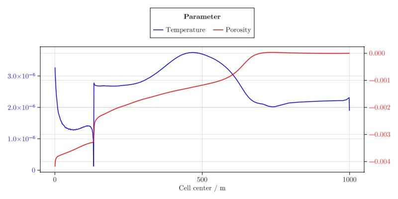

Example on GitHub

If you would like to run this example yourself, it can be downloaded from the JutulDarcy.jl GitHub repository as a script, or as a Jupyter Notebook

This page was generated using Literate.jl.

Validation of equation-of-state compositional simulator ​

Plot solutions and compare ​

Calculate sensitivities ​

Example on GitHub ​

Validation of equation-of-state compositional simulator

Plot solutions and compare

Calculate sensitivities

Example on GitHub