Gravity segregation example
The simplest type of porous media simulation problem to set up that is not trivial is the transition to equilibrium from an unstable initial condition. Placing a heavy fluid on top of a lighter fluid will lead to the heavy fluid moving down while the lighter fluid moves up.
Problem set up
We define a simple 1D gravity column with an approximate 10-1 ratio in density between the two compressible phases and let it simulate until equilibrium is reached.
using JutulDarcy, Jutul
nc = 100
Darcy, bar, kg, meter, day = si_units(:darcy, :bar, :kilogram, :meter, :day)

g = CartesianMesh((1, 1, nc), (1.0, 1.0, 10.0))
domain = reservoir_domain(g, permeability = 1.0*Darcy)
DataDomain wrapping CartesianMesh (3D) with 1x1x100=100 cells with 17 data fields added:
100 Cells
:permeability => 100 Vector{Float64}
:porosity => 100 Vector{Float64}
:rock_thermal_conductivity => 100 Vector{Float64}
:fluid_thermal_conductivity => 100 Vector{Float64}
:rock_density => 100 Vector{Float64}
:cell_centroids => 3×100 Matrix{Float64}
:volumes => 100 Vector{Float64}
99 Faces
:neighbors => 2×99 Matrix{Int64}
:areas => 99 Vector{Float64}
:normals => 3×99 Matrix{Float64}
:face_centroids => 3×99 Matrix{Float64}
198 HalfFaces
:half_face_cells => 198 Vector{Int64}
:half_face_faces => 198 Vector{Int64}
402 BoundaryFaces
:boundary_areas => 402 Vector{Float64}
:boundary_centroids => 3×402 Matrix{Float64}
:boundary_normals => 3×402 Matrix{Float64}
:boundary_neighbors => 402 Vector{Int64}Fluid properties
Define two phases liquid and vapor with a 10-1 ratio reference densities and set up the simulation model.
p0 = 100*bar
rhoLS = 1000.0*kg/meter^3
rhoVS = 100.0*kg/meter^3
cl, cv = 1e-5/bar, 1e-4/bar
L, V = LiquidPhase(), VaporPhase()
sys = ImmiscibleSystem([L, V])
model = SimulationModel(domain, sys)SimulationModel:
Model with 200 degrees of freedom, 200 equations and 498 parameters
domain:
DiscretizedDomain with MinimalTPFATopology (100 cells, 99 faces) and discretizations for mass_flow, heat_flow
system:
ImmiscibleSystem with LiquidPhase, VaporPhase
context:
DefaultContext(EquationMajorLayout(false), 9223372036854775807, 1)
formulation:
FullyImplicitFormulation()
data_domain:
DataDomain wrapping CartesianMesh (3D) with 1x1x100=100 cells with 17 data fields added:
  100 Cells
    :permeability => 100 Vector{Float64}
    :porosity => 100 Vector{Float64}
    :rock_thermal_conductivity => 100 Vector{Float64}
    :fluid_thermal_conductivity => 100 Vector{Float64}
    :rock_density => 100 Vector{Float64}
    :cell_centroids => 3×100 Matrix{Float64}
    :volumes => 100 Vector{Float64}
  99 Faces
    :neighbors => 2×99 Matrix{Int64}
    :areas => 99 Vector{Float64}
    :normals => 3×99 Matrix{Float64}
    :face_centroids => 3×99 Matrix{Float64}
  198 HalfFaces
    :half_face_cells => 198 Vector{Int64}
    :half_face_faces => 198 Vector{Int64}
  402 BoundaryFaces
    :boundary_areas => 402 Vector{Float64}
    :boundary_centroids => 3×402 Matrix{Float64}
    :boundary_normals => 3×402 Matrix{Float64}
    :boundary_neighbors => 402 Vector{Int64}
primary_variables:
1) Pressure ∈ 100 Cells: 1 dof each
2) Saturations ∈ 100 Cells: 1 dof, 2 values each
secondary_variables:
1) PhaseMassDensities ∈ 100 Cells: 2 values each
-> ConstantCompressibilityDensities as evaluator
2) TotalMasses ∈ 100 Cells: 2 values each
-> TotalMasses as evaluator
3) RelativePermeabilities ∈ 100 Cells: 2 values each
-> BrooksCoreyRelativePermeabilities as evaluator
4) PhaseMobilities ∈ 100 Cells: 2 values each
-> JutulDarcy.PhaseMobilities as evaluator
5) PhaseMassMobilities ∈ 100 Cells: 2 values each
-> JutulDarcy.PhaseMassMobilities as evaluator
parameters:
1) Transmissibilities ∈ 99 Faces: Scalar
2) TwoPointGravityDifference ∈ 99 Faces: Scalar
3) PhaseViscosities ∈ 100 Cells: 2 values each
4) FluidVolume ∈ 100 Cells: Scalar
equations:
1) mass_conservation ∈ 100 Cells: 2 values each
-> ConservationLaw{:TotalMasses, TwoPointPotentialFlowHardCoded{Vector{Int64}, Vector{@NamedTuple{self::Int64, other::Int64, face::Int64, face_sign::Int64}}}, Jutul.DefaultFlux, 2}
output_variables:
Pressure, Saturations, TotalMasses
extra:
OrderedCollections.OrderedDict{Symbol, Any} with keys: Symbol[]Definition for phase mass densities
Replace default density with a constant compressibility function that uses the reference values at the initial pressure.
density = ConstantCompressibilityDensities(sys, p0, [rhoLS, rhoVS], [cl, cv])
set_secondary_variables!(model, PhaseMassDensities = density)
Set up initial state
Put heavy phase on top and light phase on bottom. Saturations have one value per phase, per cell and consequently a per-cell instantiation will require a two by number of cells matrix as input.
nl = nc ÷ 2
sL = vcat(ones(nl), zeros(nc - nl))'
s0 = vcat(sL, 1 .- sL)
state0 = setup_state(model, Pressure = p0, Saturations = s0)
Dict{Symbol, Any} with 7 entries:
:PhaseMassMobilities => [0.0 0.0 … 0.0 0.0; 0.0 0.0 … 0.0 0.0]
:PhaseMassDensities => [0.0 0.0 … 0.0 0.0; 0.0 0.0 … 0.0 0.0]
:RelativePermeabilities => [0.5 0.5 … 0.5 0.5; 0.5 0.5 … 0.5 0.5]
:Saturations => [1.0 1.0 … 0.0 0.0; 0.0 0.0 … 1.0 1.0]
:Pressure => [1.0e7, 1.0e7, 1.0e7, 1.0e7, 1.0e7, 1.0e7, 1.0e7, …
:TotalMasses => [0.0 0.0 … 0.0 0.0; 0.0 0.0 … 0.0 0.0]
:PhaseMobilities => [0.0 0.0 … 0.0 0.0; 0.0 0.0 … 0.0 0.0]Convert time-steps from days to seconds
timesteps = repeat([0.02]*day, 150)150-element Vector{Float64}:
1728.0
1728.0
1728.0
1728.0
1728.0
1728.0
1728.0
1728.0
1728.0
1728.0
⋮
1728.0
1728.0
1728.0
1728.0
1728.0
1728.0
1728.0
1728.0
1728.0# Perform simulation
states, report = simulate(state0, model, timesteps, info_level = -1)SimResult with 150 entries:
states (model variables)
:Saturations => Matrix{Float64} of size (2, 100)
:Pressure => Vector{Float64} of size (100,)
:TotalMasses => Matrix{Float64} of size (2, 100)
reports (timing/debug information)
:ministeps => Vector{Any} of size (1,)
:total_time => Float64
:output_time => Float64
Completed at Oct. 01 2024 16:10 after 494 milliseconds, 611 microseconds, 72 nanoseconds.Plot results
The 1D nature of the problem allows us to plot all timesteps simultaneously in 2D. We see that the heavy fluid, colored blue, is initially at the top of the domain and the lighter fluid is at the bottom. These gradually switch places until all the heavy fluid is at the lower part of the column.
using GLMakie
tmp = vcat(map((x) -> x[:Saturations][1, :]', states)...)
f = Figure()
ax = Axis(f[1, 1], xlabel = "Time", ylabel = "Depth", title = "Gravity segregation")
hm = heatmap!(ax, tmp, colormap = :seismic)
Colorbar(f[1, 2], hm)
f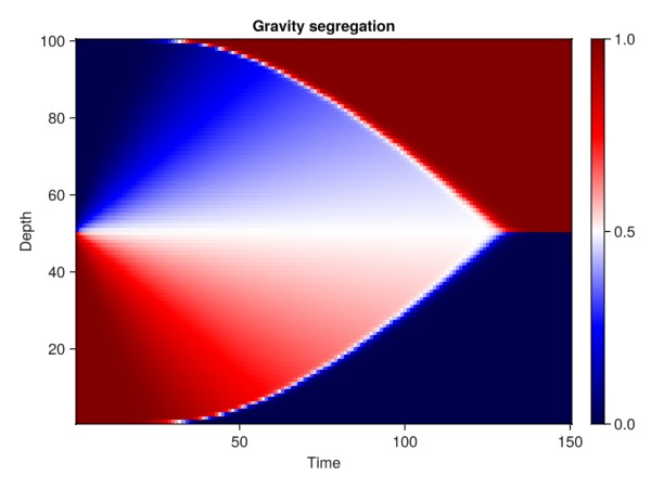
Example on GitHub
If you would like to run this example yourself, it can be downloaded from the JutulDarcy.jl GitHub repository as a script, or as a Jupyter Notebook
This page was generated using Literate.jl.