Plotting CO2 properties used in compositional model
JutulDarcy includes a set of pre-generated tables for simulation of CO2 storage in saline aquifers, as well as functions for calculating PVT and solubility properties of CO2-brine mixtures with varying degrees of salinity.
For more details on the property calculations used herein, please see the paper Three-dimensional simulation of geologic carbon dioxide sequestration using MRST by L. Saló et al (2024).
This example demonstrates how to plot the properties, and does a basic comparison of how the properties change when the aqueous phase has salts added.
using Jutul, JutulDarcy, GLMakie
import JutulDarcy.CO2Properties: co2_brine_property_tables
Define plotting functions
We define a plotting function that varies temperature, and one that compares the same property with and without salts for a given temperature.
T = [20.0, 40.0, 60.0, 80.0, 100.0]
p = range(5, 300, 100)

function plot_property(prop, tab, component, title = "")
    trans = x -> x
    if prop == :viscosity
        u = "(Pa s)"
    elseif prop == :density
        u = "(kg/m^3)"
    elseif prop == :K
        u = " (log10)"
        trans = log10
    else
        u = ""
    end
    is_h2o = component == :H2O
    fig = Figure(size = (800, 600))
    ax = Axis(fig[1, 1], title = title, xlabel = "Pressure (bar)", ylabel = "$component $prop $u")

    F = tab[prop]
    if prop == :K
        F = F.K
    end
    for (i, T_i) in enumerate(T)
        val = F.(convert_to_si(p, :bar), T_i + 273.15)
        if is_h2o
            val = map(first, val)
        else
            val = map(last, val)
        end
        lines!(ax, p, trans.(val), label = "T=$(T_i) °C",
            colormap = :hot,
            color = i,
            colorrange = (1, length(T)+3),
            linewidth = 2,
        )
    end
    axislegend(position = :lt, orientation = :horizontal)
    fig
end

function plot_brine_comparison(prop, T, tab1, tab2, component, title = "")
    trans = x -> x
    if prop == :viscosity
        u = "(Pa s)"
    elseif prop == :density
        u = "(kg/m^3)"
    elseif prop == :K
        u = ""
        u = " (log10)"
        trans = log10
    else
        u = ""
    end
    is_h2o = component == :H2O
    fig = Figure(size = (800, 600))
    ax = Axis(fig[1, 1], title = title, xlabel = "Pressure (bar)", ylabel = "$component $prop $u")

    pbar = convert_to_si.(p, :bar)

    F1 = tab1[prop]
    F2 = tab2[prop]
    if prop == :K
        F1 = F1.K
        F2 = F2.K
    end
    val1 = F1.(pbar, T + 273.15)
    val2 = F2.(pbar, T + 273.15)

    if is_h2o
        val1 = map(first, val1)
        val2 = map(first, val2)
    else
        val1 = map(last, val1)
        val2 = map(last, val2)
    end
    lines!(ax, trans.(val1), label = "Water",
        linewidth = 2,
    )
    lines!(ax, trans.(val2), label = "Brine",
        linewidth = 2,
    )
    axislegend(position = :lt, orientation = :horizontal)
    fig
end
plot_brine_comparison (generic function with 2 methods)Generate tables
We get tables for a wide pressure and temperature range. The first set of tables assumes no salts, and the second set of tables uses specified molar fractions of salts in the aqueous phase.
tab_water = co2_brine_property_tables()
tab_brine = co2_brine_property_tables(
    salt_names = ["NaCl", "KCl"],
    salt_mole_fractions = [0.05, 0.01]
)
Dict{Symbol, Any} with 11 entries:
:density => BilinearInterpolant{Vector{Float64}, Matr…
:heat_capacity_constant_pressure => BilinearInterpolant{Vector{Float64}, Matr…
:phase_conductivity => BilinearInterpolant{Vector{Float64}, Matr…
:K => KValueWrapper{BilinearInterpolant{Vector{…
:co2_table => (data = [1.0 101325.0 … 827.805 434249.0;…
:viscosity => BilinearInterpolant{Vector{Float64}, Matr…
:h2o_table => (data = [1.0 101325.0 … 4216.11 2.04082e5…
:solubility_table => (data = [1.0 101325.0 0.00660871 0.001131…
:enthalpy => BilinearInterpolant{Vector{Float64}, Matr…
:heat_capacity_constant_volume => BilinearInterpolant{Vector{Float64}, Matr…
:internal_energy => BilinearInterpolant{Vector{Float64}, Matr…Plot aqueous mass density
plot_property(:density, tab_water, :H2O, "Pure phase density, no salts")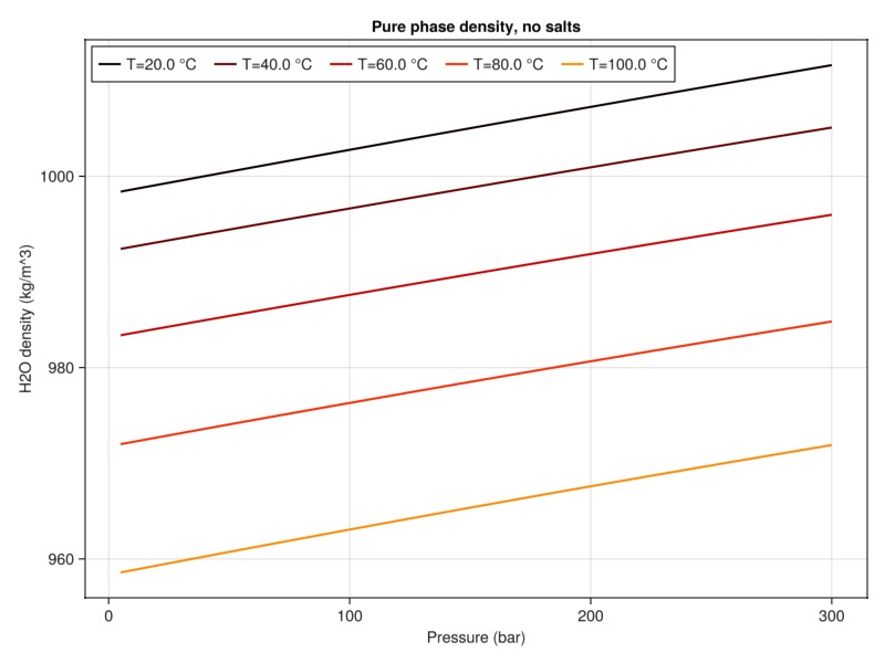
Plot gaseous mass density
plot_property(:density, tab_water, :CO2, "Pure phase density, no salts")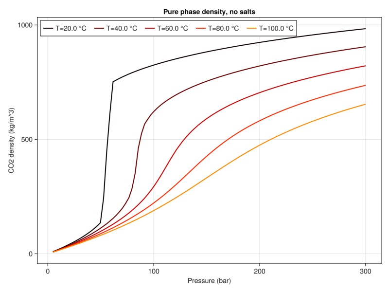
Plot aqueous viscosity
plot_property(:viscosity, tab_water, :H2O, "Pure phase viscosity, no salts")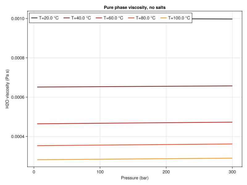
Plot gaseous viscosity
plot_property(:viscosity, tab_water, :CO2, "Pure phase viscosity, no salts")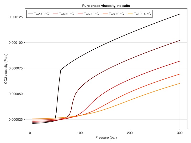
Plot K-value of CO2
The K value defines the ratio between liquid and vapor phases at equilibrium conditions and is closely related to solubility. For a component we relate the liquid mass fraction
plot_property(:K, tab_water, :CO2, "K value of CO2 component in aqueous phase, no salts")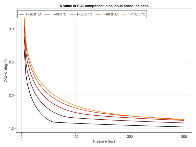
Compare viscosity with and without salts
plot_brine_comparison(:density, 30.0, tab_water, tab_brine, :H2O, "Pure phase viscosity with salts")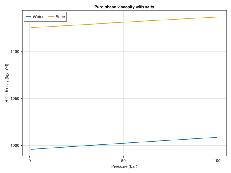
Compare K value with and without salts
plot_brine_comparison(:K, 30.0, tab_water, tab_brine, :CO2, "K value of CO2 component in aqueous phase")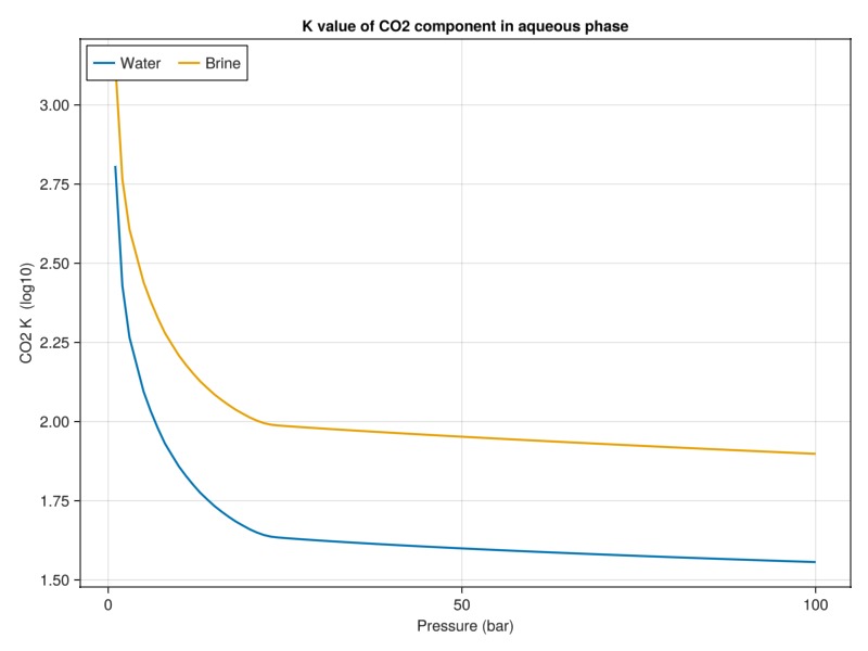
Example on GitHub
If you would like to run this example yourself, it can be downloaded from the JutulDarcy.jl GitHub repository as a script, or as a Jupyter Notebook
This page was generated using Literate.jl.