
High-enthalpy geothermal system above a magmatic intrusion
ProductionThis example demonstrates simulation of a high-enthalpy geothermal system heated by a cooling magmatic intrusion, inspired by the production and reinjection scenarios of []. The fluid is pure water, modelled with the pressure-enthalpy formulation in Fimbul (H2OSystem), so the reservoir may contain liquid, vapor, two-phase and supercritical water.
The example consists of two parts:
Natural state: A 900 °C intrusion is emplaced 2–3 km below the surface and left to develop a hydrothermal convection system for 2400 years.
Production: Starting from the natural state, we compare 100 years of production with and without reinjection of cold water.
Add required modules to namespace
using Jutul, JutulDarcy, Fimbul
using HYPRE
using GLMakie
Useful SI units
meter, year = si_units(:meter, :year);Set up the natural-state case
The domain is 10 km × 10 km × 5 km, with an ellipsoidal intrusion of horizontal radius 1.5 km centered horizontally. We use a relatively coarse tensor mesh to keep the runtime moderate. The mesh has uniform cells horizontally across the intrusion and vertically from the base of the cap rock to the bottom of the intrusion, so that the convection plume above the intrusion is resolved, and cells growing towards the domain boundaries. Fluid can flow along the wellbore of a shut well, so we simulate the natural state without wells by setting num_years = 0. The wells are added when we set up the production scenarios.
dims = (41, 41, 40)
case_args = (
    dims = dims,
    injector_position = (0.0, 0.0).*meter,
    cell_growth = 1.25,
)
case_ns = magmatic_intrusion(; case_args...,
    natural_state_time = 2400.0year,
    num_years = 0,
)
model = reservoir_model(case_ns.model)
mesh = physical_representation(model.data_domain);
Inspect the model
We first inspect the model interactively, starting with the initial temperature. Other properties can be selected in the viewer, e.g., the permeability, which shows the low-permeability cap rock covering the top 500 m of the domain. For the 3D plots in this example, we cut away the quadrant of the domain facing the viewer, so that the cut planes pass through the center of the intrusion.
xc = model.data_domain[:cell_centroids]
x_mid = sum(extrema(xc[1, :]))/2
y_mid = sum(extrema(xc[2, :]))/2
cutaway = .!(xc[1, :] .< x_mid .&& xc[2, :] .< y_mid)
axis_args = (zreversed = true, aspect = :data, perspectiveness = 0.75, elevation = π/16)
plot_res_args = (
    resolution = (1000, 800), aspect = :data,
    axis_args = axis_args,
    cells = cutaway,
    fancy = false
)
plot_reservoir(case_ns; key = :Temperature, plot_res_args...)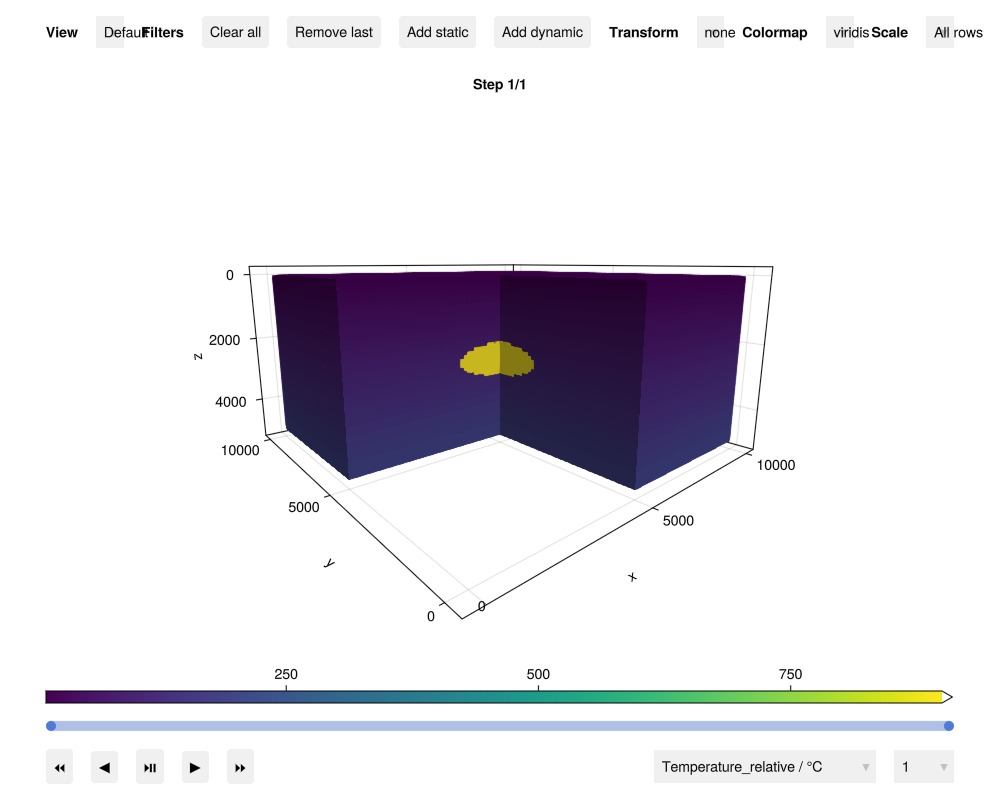
Initial temperature
The initial temperature follows a linear geothermal gradient of 37.5 °C/km, with the intrusion at 900 °C.
fig = Figure(size = (900, 700))
ax = Axis3(fig[1, 1]; title = "Initial temperature", axis_args...)
T0 = convert_from_si.(case_ns.state0[:Reservoir][:Temperature], :Celsius)
plt = plot_cell_data!(ax, mesh, T0;
    cells = cutaway, colormap = :seaborn_icefire_gradient)
Colorbar(fig[1, 2], plt; label = "T (°C)")
fig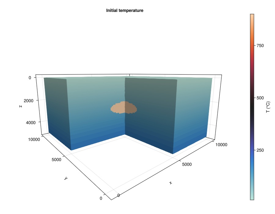
Simulate the natural state
We use the same solver settings for all simulations in this example: we remove the default maximum timestep of one year, since the system evolves slowly once the convection pattern is established, use relaxation of the Newton updates, and use slightly relaxed convergence tolerances. Close to the critical point of water, the fluid properties change rapidly, and these settings help the nonlinear solver through this region. We also limit the change in enthalpy per timestep.
Note that the natural-state simulation takes a while to run. The early, transient part of the simulation, when the intrusion cools and a two-phase region develops above it, requires many short timesteps. Once the convection pattern is established, the timesteps increase.
function run_case(case)
    sim, cfg = setup_reservoir_simulator(case;
        max_timestep = Inf,
        relaxation = true,
        tol_cnv = 1e-2,
        tol_mb = 1e-5,
        info_level = 0
    )
    tss = VariableChangeTimestepSelector(:Enthalpy, 1e5;
    relative = false, model = :Reservoir)
    push!(cfg[:timestep_selectors], tss)
    return simulate_reservoir(case; simulator = sim, config = cfg)
end

results_ns = run_case(case_ns);
Jutul: Simulating 2400 years as 24 report steps
┌ Warning: Pressure: 67240 non-finite values found. Indices: (limited to 10) [1, 2, 3, 4, 5, 6, 7, 8, 9, 10], values: [NaN, NaN, NaN, NaN, NaN, NaN, NaN, NaN, NaN, NaN]
└ @ Jutul ~/.julia/packages/Jutul/9NQ66/src/utils.jl:95
┌ Warning: Pressure: 67240 non-finite values found. Indices: (limited to 10) [1, 2, 3, 4, 5, 6, 7, 8, 9, 10], values: [NaN, NaN, NaN, NaN, NaN, NaN, NaN, NaN, NaN, NaN]
└ @ Jutul ~/.julia/packages/Jutul/9NQ66/src/utils.jl:95
┌ Warning: Pressure: 67240 non-finite values found. Indices: (limited to 10) [1, 2, 3, 4, 5, 6, 7, 8, 9, 10], values: [NaN, NaN, NaN, NaN, NaN, NaN, NaN, NaN, NaN, NaN]
└ @ Jutul ~/.julia/packages/Jutul/9NQ66/src/utils.jl:95
┌ Warning: Pressure: 67240 non-finite values found. Indices: (limited to 10) [1, 2, 3, 4, 5, 6, 7, 8, 9, 10], values: [NaN, NaN, NaN, NaN, NaN, NaN, NaN, NaN, NaN, NaN]
└ @ Jutul ~/.julia/packages/Jutul/9NQ66/src/utils.jl:95
┌ Warning: Pressure: 67240 non-finite values found. Indices: (limited to 10) [1, 2, 3, 4, 5, 6, 7, 8, 9, 10], values: [NaN, NaN, NaN, NaN, NaN, NaN, NaN, NaN, NaN, NaN]
└ @ Jutul ~/.julia/packages/Jutul/9NQ66/src/utils.jl:95
┌ Warning: Pressure: 67240 non-finite values found. Indices: (limited to 10) [1, 2, 3, 4, 5, 6, 7, 8, 9, 10], values: [NaN, NaN, NaN, NaN, NaN, NaN, NaN, NaN, NaN, NaN]
└ @ Jutul ~/.julia/packages/Jutul/9NQ66/src/utils.jl:95
┌ Warning: Pressure: 67240 non-finite values found. Indices: (limited to 10) [1, 2, 3, 4, 5, 6, 7, 8, 9, 10], values: [NaN, NaN, NaN, NaN, NaN, NaN, NaN, NaN, NaN, NaN]
└ @ Jutul ~/.julia/packages/Jutul/9NQ66/src/utils.jl:95
┌ Warning: Pressure: 67240 non-finite values found. Indices: (limited to 10) [1, 2, 3, 4, 5, 6, 7, 8, 9, 10], values: [NaN, NaN, NaN, NaN, NaN, NaN, NaN, NaN, NaN, NaN]
└ @ Jutul ~/.julia/packages/Jutul/9NQ66/src/utils.jl:95
┌ Warning: Pressure: 67240 non-finite values found. Indices: (limited to 10) [1, 2, 3, 4, 5, 6, 7, 8, 9, 10], values: [NaN, NaN, NaN, NaN, NaN, NaN, NaN, NaN, NaN, NaN]
└ @ Jutul ~/.julia/packages/Jutul/9NQ66/src/utils.jl:95
┌ Warning: Pressure: 67240 non-finite values found. Indices: (limited to 10) [1, 2, 3, 4, 5, 6, 7, 8, 9, 10], values: [NaN, NaN, NaN, NaN, NaN, NaN, NaN, NaN, NaN, NaN]
└ @ Jutul ~/.julia/packages/Jutul/9NQ66/src/utils.jl:95
┌ Warning: Pressure: 67240 non-finite values found. Indices: (limited to 10) [1, 2, 3, 4, 5, 6, 7, 8, 9, 10], values: [NaN, NaN, NaN, NaN, NaN, NaN, NaN, NaN, NaN, NaN]
└ @ Jutul ~/.julia/packages/Jutul/9NQ66/src/utils.jl:95
┌ Warning: Pressure: 67240 non-finite values found. Indices: (limited to 10) [1, 2, 3, 4, 5, 6, 7, 8, 9, 10], values: [NaN, NaN, NaN, NaN, NaN, NaN, NaN, NaN, NaN, NaN]
└ @ Jutul ~/.julia/packages/Jutul/9NQ66/src/utils.jl:95
┌ Warning: Pressure: 67240 non-finite values found. Indices: (limited to 10) [1, 2, 3, 4, 5, 6, 7, 8, 9, 10], values: [NaN, NaN, NaN, NaN, NaN, NaN, NaN, NaN, NaN, NaN]
└ @ Jutul ~/.julia/packages/Jutul/9NQ66/src/utils.jl:95
┌ Warning: Pressure: 67240 non-finite values found. Indices: (limited to 10) [1, 2, 3, 4, 5, 6, 7, 8, 9, 10], values: [NaN, NaN, NaN, NaN, NaN, NaN, NaN, NaN, NaN, NaN]
└ @ Jutul ~/.julia/packages/Jutul/9NQ66/src/utils.jl:95
┌ Warning: Pressure: 67240 non-finite values found. Indices: (limited to 10) [1, 2, 3, 4, 5, 6, 7, 8, 9, 10], values: [NaN, NaN, NaN, NaN, NaN, NaN, NaN, NaN, NaN, NaN]
└ @ Jutul ~/.julia/packages/Jutul/9NQ66/src/utils.jl:95
╭────────────────┬──────────┬────────────────┬──────────────╮
│ Iteration type │ Avg/step │ Avg/ministep │ Total │
│ │ 24 steps │ 1563 ministeps │ (wasted) │
├────────────────┼──────────┼────────────────┼──────────────┤
│ Newton │ 222.167 │ 3.41139 │ 5332 (917) │
│ Linearization │ 286.667 │ 4.40179 │ 6880 (975) │
│ Linear solver │ 484.833 │ 7.44466 │ 11636 (2459) │
│ Precond apply │ 969.667 │ 14.8893 │ 23272 (4918) │
╰────────────────┴──────────┴────────────────┴──────────────╯
╭───────────────┬──────────┬────────────┬──────────╮
│ Timing type │ Each │ Relative │ Total │
│ │ ms │ Percentage │ s │
├───────────────┼──────────┼────────────┼──────────┤
│ Properties │ 13.1557 │ 9.02 % │ 70.1463 │
│ Equations │ 21.5685 │ 19.09 % │ 148.3912 │
│ Assembly │ 4.4827 │ 3.97 % │ 30.8410 │
│ Linear solve │ 5.8931 │ 4.04 % │ 31.4219 │
│ Linear setup │ 59.0795 │ 40.53 % │ 315.0118 │
│ Precond apply │ 4.9313 │ 14.76 % │ 114.7614 │
│ Update │ 1.0467 │ 0.72 % │ 5.5812 │
│ Convergence │ 6.4939 │ 5.75 % │ 44.6780 │
│ Input/Output │ 0.0858 │ 0.02 % │ 0.1341 │
│ Other │ 3.0681 │ 2.10 % │ 16.3592 │
├───────────────┼──────────┼────────────┼──────────┤
│ Total │ 145.7851 │ 100.00 % │ 777.3261 │
╰───────────────┴──────────┴────────────┴──────────╯Interactive visualization of the natural state
The interactive viewer shows the temperature at each report step of the natural state. Filtering out low temperatures shows how the hot plume develops above the intrusion.
plot_reservoir(case_ns.model, results_ns.states;
    key = :Temperature, colormap = :seaborn_icefire_gradient, cells = cutaway, plot_res_args...)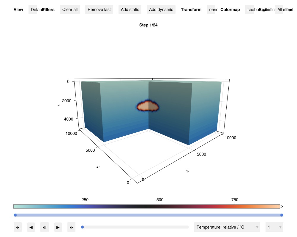
Development of the convection plume
The hot intrusion heats the surrounding water, which rises buoyantly and is replaced by colder water flowing in from the sides. We plot the temperature (top) and liquid saturation (bottom) at selected times.
t_ns = cumsum(case_ns.dt)
nearest_step(t) = argmin(abs.(t_ns .- t))
plot_times = [300.0, 600.0, 1200.0].*year
T_range = (10.0, 900.0)
fig = Figure(size = (1200, 750))
for (i, t) in enumerate(plot_times)
    step = nearest_step(t)
    T = convert_from_si.(results_ns.states[step][:Temperature], :Celsius)
    ax = Axis3(fig[1, i];
        title = "$(round(Int, t_ns[step]/year)) years", axis_args...)
    plot_cell_data!(ax, mesh, T; cells = cutaway,
        colormap = :seaborn_icefire_gradient, colorrange = T_range)
    hidedecorations!(ax)
    S = results_ns.states[step][:Saturations][1, :]
    ax = Axis3(fig[2, i]; axis_args...)
    plot_cell_data!(ax, mesh, S; cells = cutaway,
        colormap = :gray1, colorrange = (0.0, 1.0))
    hidedecorations!(ax)
end
Colorbar(fig[1, length(plot_times) + 1]; colormap = :seaborn_icefire_gradient,
    colorrange = T_range, label = "T (°C)")
Colorbar(fig[2, length(plot_times) + 1]; colormap = :gray1,
    colorrange = (0.0, 1.0), label = "Liquid saturation")
fig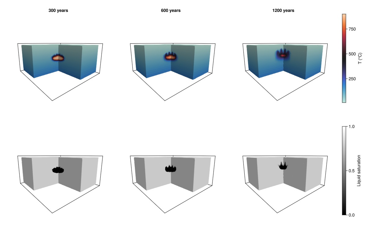
Phase diagram
The evolution of the fluid can be shown in a pressure-enthalpy phase diagram, with temperature contours and the two-phase envelope. We follow four cells on the vertical line through the center of the intrusion: one at the center of the intrusion, one just above it, one higher up in the convection plume, and one near the surface. Each line shows the state of one cell at every report step of the natural state (circles), starting from the initial state (star). Early in the natural state, the fluid passes close to the critical point of water (22.064 MPa, 2.085 MJ/kg), where the fluid properties change rapidly. This is the most challenging part of the simulation.
x_c = (x_mid, y_mid)
probe_depths = [2500.0, 1900.0, 1300.0, 700.0].*meter
probe_cells = [argmin((xc[1, :] .- x_c[1]).^2 .+ (xc[2, :] .- x_c[2]).^2 .+
    (xc[3, :] .- d).^2) for d in probe_depths]
probe_labels = ["Intrusion center", "Above intrusion", "Upper plume", "Near surface"]
probe_colors = [:red, :lightgreen, :cyan, :magenta]
states_ph = vcat([case_ns.state0[:Reservoir]], results_ns.states)
tables = model.system.pvt_tables
fig = Figure(size = (900, 650), fontsize = 14)
ax = Axis(fig[1, 1])
handles = plot_phase_diagram_contours!(ax, tables;
    pressure_limits = (0.0, 30e6), enthalpy_limits = (0.0, 4.5e6), lines = true)
for (i, (c, label)) in enumerate(zip(probe_cells, probe_labels))
    h = [state[:Enthalpy][c] for state in states_ph]./1e3
    p = [state[:Pressure][c] for state in states_ph]./1e6
    depth = round(Int, xc[3, c])
    lines!(ax, h, p; color = probe_colors[i], linewidth = 3, label = "$label ($depth m)")
    scatter!(ax, h, p; color = probe_colors[i], markersize = 10,
        strokecolor = :black, strokewidth = 1)
    scatter!(ax, h[1:1], p[1:1]; color = :yellow, markersize = 12,
        strokecolor = :black, strokewidth = 1, marker = :star5)
end

axislegend(ax; position = :rb)
Colorbar(fig[1, 2], handles.filled; label = "T (°C)")
fig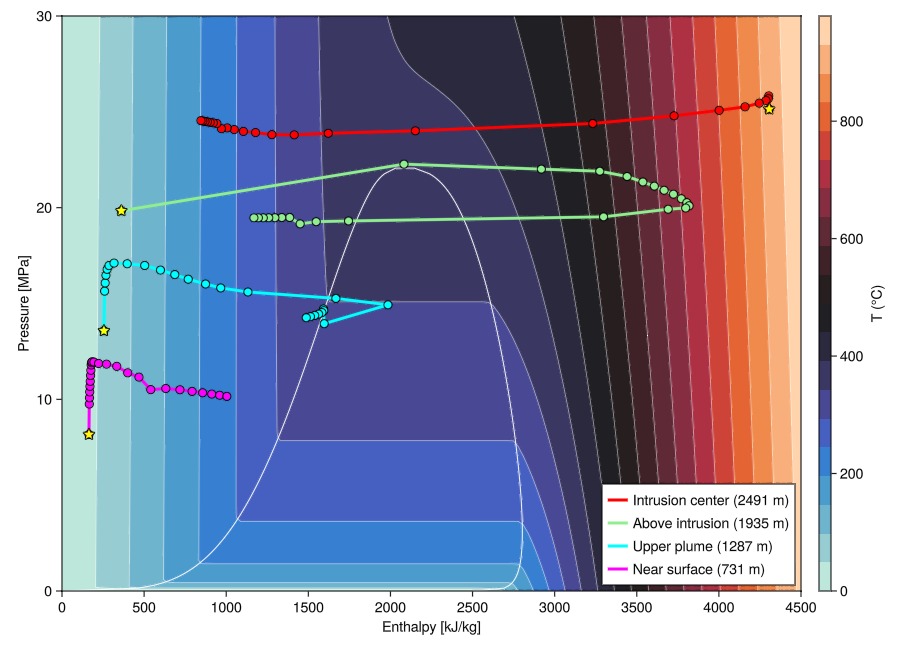
Production scenarios
We set up the production scenarios with wells, starting from the end of the natural state (initial_state), and simulate 100 years of production. The wells are multisegment wells that extend from the surface, and the well pressures are prescribed at the wellhead. The producer is open between 750 and 1750 m depth, above the intrusion, and is operated at a wellhead pressure of 10 bar. In the second scenario, cold water (80 °C) is reinjected at a wellhead pressure of 80 bar in an injector that is open between 1750 and 1950 m depth, just above the intrusion. With injection_years = 0, the injector is not included in the model. We use report steps of one year.
state_ns = results_ns.states[end]
case_inj = magmatic_intrusion(; case_args...,
    natural_state_time = 0.0,
    num_years = 100,
    report_interval = 1.0year,
    initial_state = state_ns,
)
case_noinj = magmatic_intrusion(; case_args...,
    natural_state_time = 0.0,
    num_years = 100,
    injection_years = 0,
    report_interval = 1.0year,
    initial_state = state_ns,
)
wells = get_model_wells(case_inj.model)
function plot_wells!(ax)
    for well in values(wells)
        plot_well!(ax, mesh, well;
            color = :black, linewidth = 3, markersize = 0.0, fontsize = 0.0)
    end
end
plot_wells! (generic function with 1 method)Simulate
results_noinj = run_case(case_noinj);
results_inj = run_case(case_inj);
Jutul: Simulating 100 years as 100 report steps
╭────────────────┬───────────┬───────────────┬────────────╮
│ Iteration type │ Avg/step │ Avg/ministep │ Total │
│ │ 100 steps │ 252 ministeps │ (wasted) │
├────────────────┼───────────┼───────────────┼────────────┤
│ Newton │ 6.49 │ 2.5754 │ 649 (90) │
│ Linearization │ 9.01 │ 3.5754 │ 901 (96) │
│ Linear solver │ 8.58 │ 3.40476 │ 858 (95) │
│ Precond apply │ 17.16 │ 6.80952 │ 1716 (190) │
╰────────────────┴───────────┴───────────────┴────────────╯
╭───────────────┬──────────┬────────────┬──────────╮
│ Timing type │ Each │ Relative │ Total │
│ │ ms │ Percentage │ s │
├───────────────┼──────────┼────────────┼──────────┤
│ Properties │ 14.5887 │ 7.50 % │ 9.4681 │
│ Equations │ 52.2759 │ 37.33 % │ 47.1006 │
│ Assembly │ 6.1421 │ 4.39 % │ 5.5340 │
│ Linear solve │ 4.9302 │ 2.54 % │ 3.1997 │
│ Linear setup │ 56.1000 │ 28.86 % │ 36.4089 │
│ Precond apply │ 5.0504 │ 6.87 % │ 8.6665 │
│ Update │ 2.8163 │ 1.45 % │ 1.8278 │
│ Convergence │ 11.2409 │ 8.03 % │ 10.1280 │
│ Input/Output │ 0.8845 │ 0.18 % │ 0.2229 │
│ Other │ 5.5568 │ 2.86 % │ 3.6063 │
├───────────────┼──────────┼────────────┼──────────┤
│ Total │ 194.3957 │ 100.00 % │ 126.1628 │
╰───────────────┴──────────┴────────────┴──────────╯
Jutul: Simulating 100 years as 100 report steps
╭────────────────┬───────────┬───────────────┬────────────╮
│ Iteration type │ Avg/step │ Avg/ministep │ Total │
│ │ 100 steps │ 233 ministeps │ (wasted) │
├────────────────┼───────────┼───────────────┼────────────┤
│ Newton │ 6.08 │ 2.60944 │ 608 (75) │
│ Linearization │ 8.41 │ 3.60944 │ 841 (80) │
│ Linear solver │ 8.2 │ 3.51931 │ 820 (85) │
│ Precond apply │ 16.4 │ 7.03863 │ 1640 (170) │
╰────────────────┴───────────┴───────────────┴────────────╯
╭───────────────┬──────────┬────────────┬─────────╮
│ Timing type │ Each │ Relative │ Total │
│ │ ms │ Percentage │ s │
├───────────────┼──────────┼────────────┼─────────┤
│ Properties │ 14.6192 │ 9.67 % │ 8.8884 │
│ Equations │ 31.2626 │ 28.60 % │ 26.2918 │
│ Assembly │ 4.8745 │ 4.46 % │ 4.0995 │
│ Linear solve │ 4.7256 │ 3.13 % │ 2.8732 │
│ Linear setup │ 52.8059 │ 34.92 % │ 32.1060 │
│ Precond apply │ 4.9792 │ 8.88 % │ 8.1660 │
│ Update │ 1.2743 │ 0.84 % │ 0.7748 │
│ Convergence │ 7.6890 │ 7.03 % │ 6.4664 │
│ Input/Output │ 0.4773 │ 0.12 % │ 0.1112 │
│ Other │ 3.5409 │ 2.34 % │ 2.1529 │
├───────────────┼──────────┼────────────┼─────────┤
│ Total │ 151.2009 │ 100.00 % │ 91.9301 │
╰───────────────┴──────────┴────────────┴─────────╯Well performance
The produced fluid boils as it rises in the producer, and reaches the wellhead as a mixture of water and steam. The production temperature is therefore fixed at the saturation temperature at the wellhead pressure of 10 bar (about 180 °C) throughout the simulation. The specific enthalpy of the produced fluid, which determines the steam fraction, varies only slightly. We therefore show the power output, computed as the produced mass rate times the specific enthalpy of the produced fluid, which closely follows the production rate. The power output drops quickly in the first years as the pressure around the producer declines. Reinjection supports the reservoir pressure, which sustains a higher production rate and power output.
fig = Figure(size = (800, 450))
ax = Axis(fig[1, 1]; xlabel = "Time (years)", ylabel = "Power output (MW)")
colors = Makie.wong_colors()
for (i, (res, label)) in enumerate(zip(
        [results_noinj, results_inj], ["Production only", "With reinjection"]))
    t = res.time./year
    q = -res.wells[:Producer][:mass_rate]
    h = [state[:Producer][:Enthalpy][1] for state in res.result.states]
    lines!(ax, t, q.*h./1e6; color = colors[i], linewidth = 2, label = label)
end
axislegend(ax; position = :rt)
fig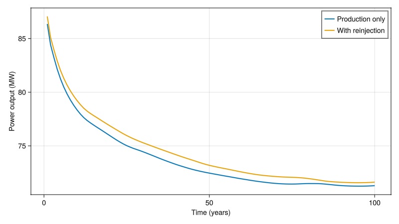
Interactive visualization of temperature changes
The interactive viewer shows the temperature change relative to the natural state for the scenario with reinjection. Filtering out values close to zero shows the cold zone developing around the injector.
Δstates_inj = JutulDarcy.delta_state(results_inj.states, results_ns.states[end])
plot_reservoir(case_inj.model, Δstates_inj;
    key = :Temperature, colormap = :seaborn_icefire_gradient,
    well_color = :black,
    well_arg = (markersize = 0.0,),
    step = length(Δstates_inj),
    plot_res_args...)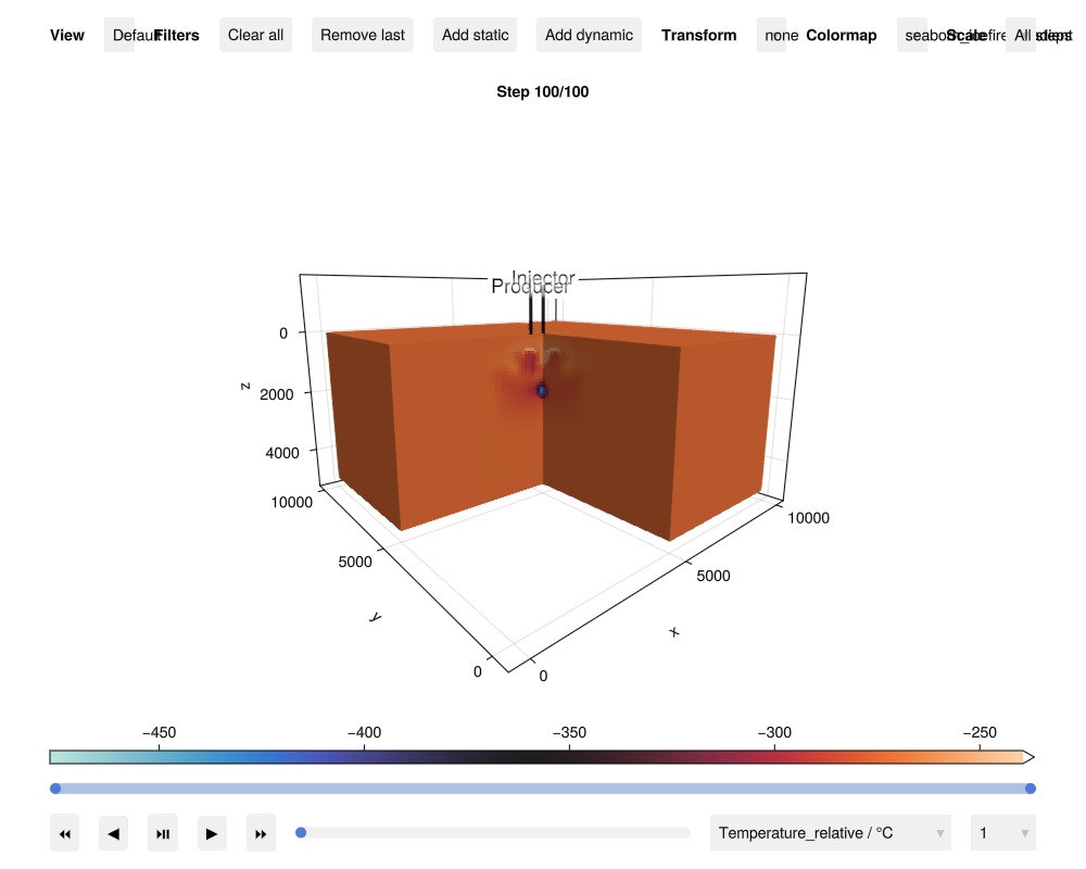
Reservoir temperature change
Finally, we plot the temperature change relative to the natural state for the scenario without (left) and with (right) reinjection. The region along the producer cools, while hot fluid drawn up from the plume warms the rock next to it. Reinjection creates a cold zone around the injector.
T_ns = results_ns.states[end][:Temperature]
results_prod = (results_noinj, results_inj)
ΔT_all = [res.states[end][:Temperature] .- T_ns for res in results_prod]
ΔT_max = maximum(maximum.(ΔT_all))
ΔT_min = minimum(minimum.(ΔT_all))
ΔT_range = (ΔT_min, ΔT_max)
(-203.4619642789869, 31.513450283948714)Diverging colormap with the neutral (white) color at ΔT = 0: the negative and positive parts of the range are mapped to the two halves of the colormap.
vik = cgrad(:vik)
ΔT_cmap = map(range(ΔT_min, ΔT_max, length = 256)) do v
    v < 0 ? vik[0.5*(v - ΔT_min)/(0 - ΔT_min)] : vik[0.5 + 0.5*v/ΔT_max]
end
fig = Figure(size = (1000, 600))
for (i, (res, ΔT, title)) in enumerate(zip(results_prod, ΔT_all,
        ["Production only", "With reinjection"]))
    ax = Axis3(fig[1, i]; title = title, axis_args...)
    plot_cell_data!(ax, mesh, ΔT; cells = cutaway,
        colormap = ΔT_cmap, colorrange = ΔT_range)
    plot_wells!(ax)
    hidedecorations!(ax)
end
Colorbar(fig[2, 1:2];
    colormap = ΔT_cmap, colorrange = ΔT_range,
    vertical = false,
    label = "ΔT (°C)")
fig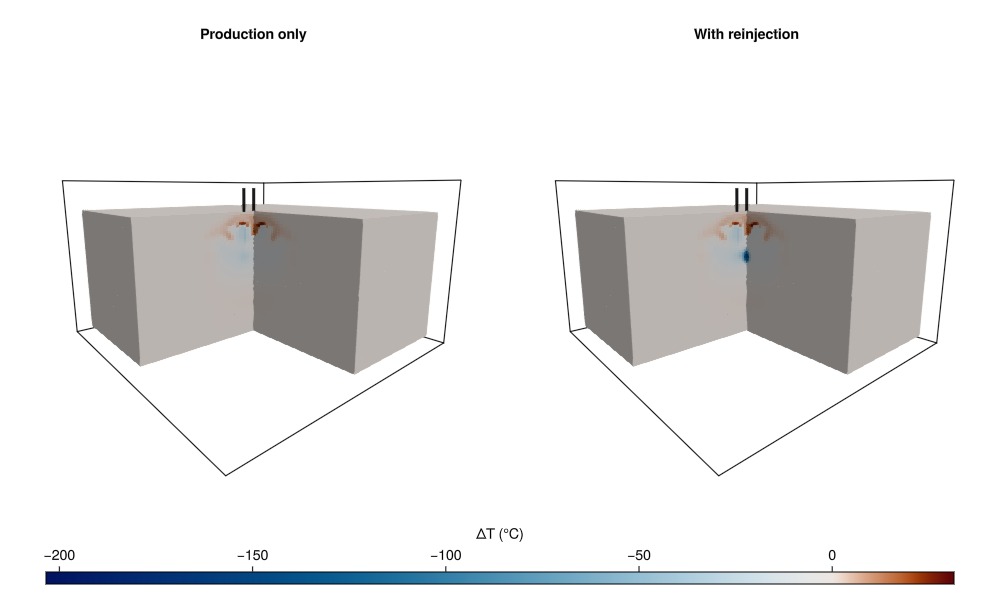
Example on GitHub
If you would like to run this example yourself, it can be downloaded from the Fimbul.jl GitHub repository as a script.
This example took 1087.938728448 seconds to complete.This page was generated using Literate.jl.