Fractured Thermal Energy Storage (FTES)
Storage FTESThis example demonstrates how to set up and simulate a Fractured Thermal Energy Storage (FTES) system using Fimbul. FTES systems exploit natural or induced fractures in low-permeability rock to store and recover thermal energy by circulating water through a fracture network connected by an injector– producer arrangement.
Our system consists of one central injector surrounded by multiple producer wells. Horizontal fracture planes connect the injector to the producers, enabling thermal transport through the fracture network even in tight rock. During charging, hot water is injected through the central well and produced at the outer producers; during discharging the flow direction is reversed.
using Jutul, JutulDarcy, Fimbul
using HYPRE
using Random
using GLMakie
Set up simulation case
We create an FTES system with 8 producer wells arranged in a circle of 35 m radius around the central injector. The wells extend to 300 m depth and the fracture network consists of 25 near-horizontal fractures distributed within the well interval. The system is charged from April to November and discharged from December to March over a 3-year period.
Random.seed!(20260225)
T_charge = convert_to_si(95, :Celsius)
T_discharge = convert_to_si(20, :Celsius)
case = Fimbul.ftes(
    (num_producers = 8, radius = 35.0, depth = 300.0),
    (num = 25, z_min = 50.0, z_max = 290.0, radius = 75.0),;
    rate_charge = 50si"litre/second",
    temperature_charge = T_charge,
    temperature_discharge = T_discharge,
    charge_period = ["April", "November"],
    discharge_period = ["December", "March"],
    utes_schedule_args = (num_years = 3,),
    info_level = 1,
);
[ Info: Setting up wells and making mesh
[ Info: Adding fractures to the mesh
[ Info: Setting up DFM model
[ Info: Setting up initial state, boundary conditions, and well controlsVisualize the FTES system
We first inspect the computational mesh and the embedded fracture network. The fracture mesh (gray surfaces) captures the codimension-one fracture planes that are resolved inside the 3D matrix mesh.
matrix_mesh = physical_representation(reservoir_model(case.model).data_domain)
fracture_mesh = physical_representation(case.model.models[:Fractures].data_domain)

axis_args = (perspectiveness = 0.75, zreversed = true, aspect = :data,
    elevation = 0.025π, azimuth = 1.35π)
fig = Figure(size = (900, 700))
ax = Axis3(fig[1, 1]; axis_args...,
    title = "FTES system: matrix mesh and fracture network")
Jutul.plot_mesh!(ax, fracture_mesh; color = :gray)
Jutul.plot_mesh_edges!(ax, matrix_mesh; alpha = 0.1)
colors = Makie.wong_colors(6)[[2,6]]

function plot_ftes_wells(ax)
    for (i, xw) in enumerate(case.input_data[:well_coordinates])
        color = ifelse(i == 1, colors[1], colors[2])
        lines!(ax, xw[1,:], xw[2,:],  xw[3,:],
            color = color, linewidth = 3)
    end
end
plot_ftes_wells(ax)
fig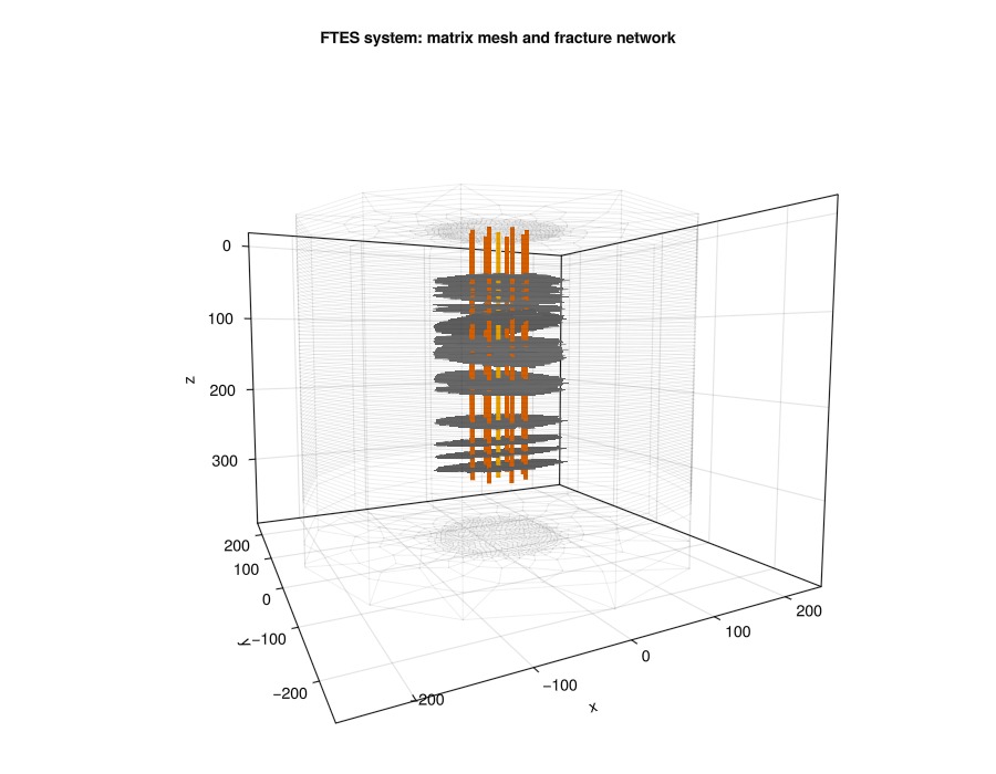
Set up reservoir simulator
We configure solver tolerances suited to the thermal DFM system. The ControlChangeTimestepSelector is used to take very small steps when well controls switch between charging and discharging to maintain convergence to aid the nonlinear solver.
simulator, config = setup_reservoir_simulator(case;
    initial_dt = 5.0,
    output_substates = true,
    relaxation = true,
);

sel = JutulDarcy.ControlChangeTimestepSelector(case.model, 0.1, 60.0)
push!(config[:timestep_selectors], sel)
sel_T = VariableChangeTimestepSelector(:Temperature, 20.0; model = :Fractures, relative = false)
push!(config[:timestep_selectors], sel_T)
config[:timestep_max_decrease] = 1e-6;
Simulate the FTES system
results = simulate_reservoir(case;
    simulator = simulator, config = config, info_level = 0);
Jutul: Simulating 3 years, 6.54 hours as 30 report steps
╭────────────────┬──────────┬───────────────┬────────────╮
│ Iteration type │ Avg/step │ Avg/ministep │ Total │
│ │ 30 steps │ 302 ministeps │ (wasted) │
├────────────────┼──────────┼───────────────┼────────────┤
│ Newton │ 54.8 │ 5.44371 │ 1644 (15) │
│ Linearization │ 64.8667 │ 6.44371 │ 1946 (16) │
│ Linear solver │ 181.4 │ 18.0199 │ 5442 (36) │
│ Precond apply │ 362.8 │ 36.0397 │ 10884 (72) │
╰────────────────┴──────────┴───────────────┴────────────╯
╭───────────────┬──────────┬────────────┬──────────╮
│ Timing type │ Each │ Relative │ Total │
│ │ ms │ Percentage │ s │
├───────────────┼──────────┼────────────┼──────────┤
│ Properties │ 10.3385 │ 3.04 % │ 16.9965 │
│ Equations │ 67.5597 │ 23.48 % │ 131.4713 │
│ Assembly │ 13.2156 │ 4.59 % │ 25.7175 │
│ Linear solve │ 17.4346 │ 5.12 % │ 28.6624 │
│ Linear setup │ 146.9805 │ 43.16 % │ 241.6359 │
│ Precond apply │ 9.7196 │ 18.89 % │ 105.7884 │
│ Update │ 2.1216 │ 0.62 % │ 3.4880 │
│ Convergence │ 1.3308 │ 0.46 % │ 2.5897 │
│ Input/Output │ 0.0894 │ 0.00 % │ 0.0270 │
│ Other │ 2.1517 │ 0.63 % │ 3.5375 │
├───────────────┼──────────┼────────────┼──────────┤
│ Total │ 340.5804 │ 100.00 % │ 559.9142 │
╰───────────────┴──────────┴────────────┴──────────╯Visualize results
Interactive inspection of matrix temperature distribution
msh = physical_representation(reservoir_model(case.model).data_domain)
geo = tpfv_geometry(msh)
x_range = diff(vcat(extrema(geo.cell_centroids[1, :])...))[1]
y_range = diff(vcat(extrema(geo.cell_centroids[2, :])...))[1]
z_range = diff(vcat(extrema(geo.cell_centroids[3, :])...))[1]
aspect  = (x_range, y_range, z_range) ./ max.(x_range, y_range, z_range)

states, dt, _ = Jutul.expand_to_ministeps(results.result)
states_m = [s[:Reservoir] for s in states]
plot_reservoir(case.model, states_m;
    key = :Temperature,
    aspect = aspect,
    colormap = :seaborn_icefire_gradient)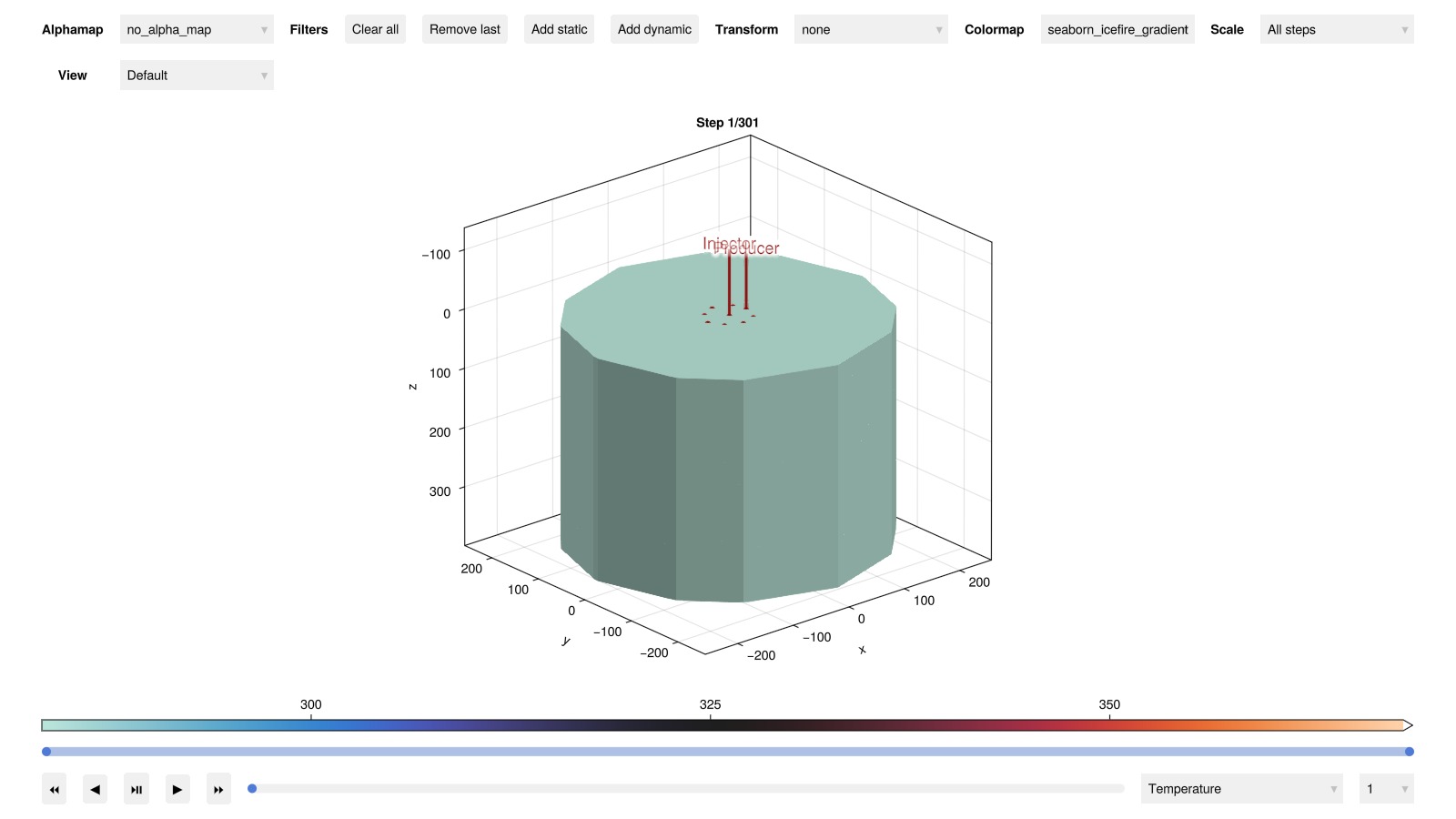
Fracture temperature distribution
The fractures are the primary heat transport pathway. We also interactively visualize the temperature field on the fracture mesh at the end of the simulation.
states_f = [s[:Fractures] for s in states]
plot_reservoir(case.model.models[:Fractures], states_f;
    key = :Temperature,
    aspect = aspect,
    colormap = :seaborn_icefire_gradient)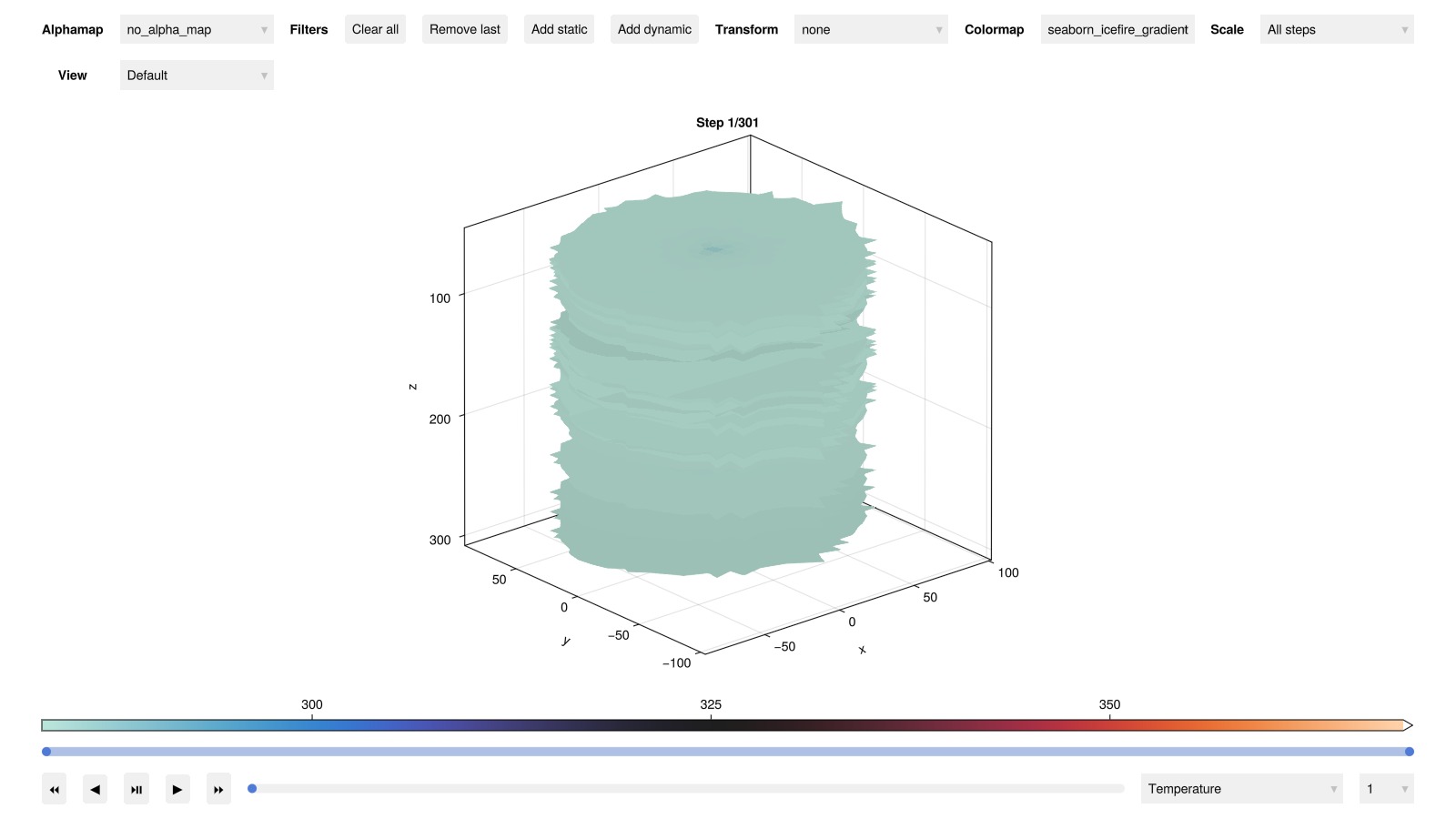
Well performance over time
Plot injection/production temperatures and flow rates throughout the operational schedule to assess thermal efficiency and system performance.
plot_well_results(results.wells, field = :temperature)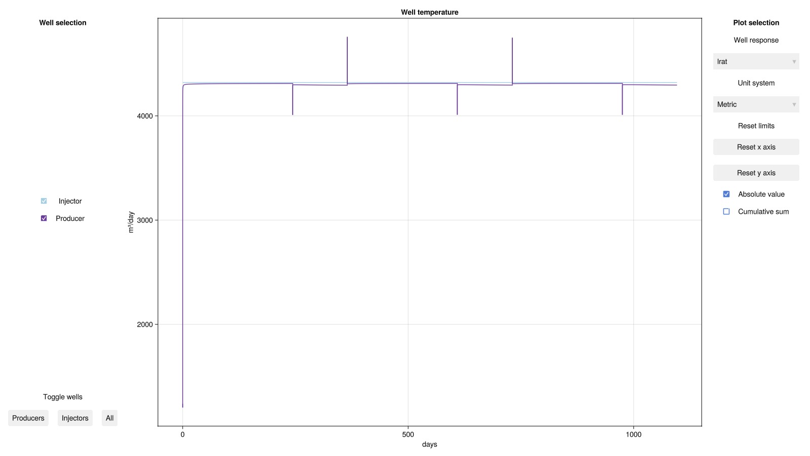
Plot Reservoir temperature at selected time steps
We visualize the temperature distribution in the reservoir after the first and last charing and discharging cycles
Extract timesteps after each charing and discharging cycle
using Dates
timestamps = case.input_data[:timestamps][2:end]

steps = findall([Dates.monthname(t) ∈ ["December", "April"] .&&
    Dates.day(t) == 1 for t in timestamps])
steps = steps[[1, 2, end-1, end]] # Select first two and last two cycles for better visualization
cells = .!(geo.cell_centroids[1,:] .< 0.0 .&& geo.cell_centroids[2,:] .< 0.0)
colorrange = convert_from_si.((T_discharge, T_charge), :Celsius)
fig = Figure(size = (800, 900))
for (k, step) in enumerate(steps)
    row = (k-1)÷2 + 1
    col = (k-1)%2 + 1
    month = Dates.monthname(case.input_data[:timestamps][step])
    year = Dates.year(case.input_data[:timestamps][step])
    ax = Axis3(fig[row, col];
        title = "$month $year",
        zreversed = true, aspect = aspect, axis_args...,
        azimuth = 1.25π, titlegap = -50)
    T = convert_from_si.(results.result.states[step][:Reservoir][:Temperature], :Celsius)
    plot_cell_data!(ax, msh, T;
        cells = cells, colormap = :seaborn_icefire_gradient, colorrange = colorrange)
    hidedecorations!(ax)
end
Colorbar(fig[3, 1:2];
    colormap = :seaborn_icefire_gradient, colorrange = colorrange,
    label = "Temperature (°C)", vertical = false, flipaxis = false)
colgap!(fig.layout, 0)
rowgap!(fig.layout, 0)
fig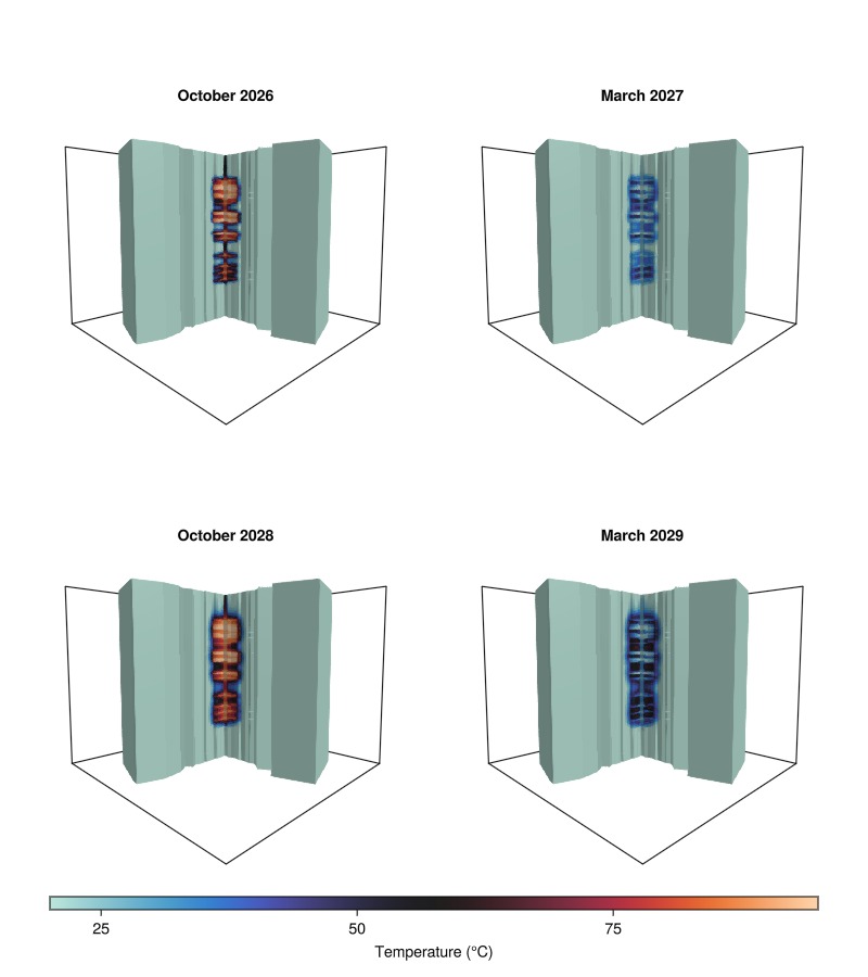
Example on GitHub
If you would like to run this example yourself, it can be downloaded from the Fimbul.jl GitHub repository as a script.
This example took 634.312339105 seconds to complete.This page was generated using Literate.jl.