Advanced Geothermal System (AGS)

This example demonstrates simulation and analysis of energy production from an Advanced Geothermal System (AGS). AGS technology utilizes closed-loop circulation systems to extract geothermal energy from deep hot rock formations, offering a novel approach to geothermal energy extraction that doesn't require natural permeability or fracture stimulation.

The AGS well setup for this example was provided by Alexander Rath (OMV)

Add required modules to namespace

using Jutul, JutulDarcy, Fimbul # Core reservoir simulation framework
using HYPRE # High-performance linear solvers
using GLMakie # 3D visualization and plotting capabilities

Useful SI units

meter, hour, day, watt = si_units(:meter, :hour, :day, :watt);

AGS setup

We consider an AGS system featuring a closed-loop configuration with a single vertical well extending 2400 m deep, followed by two horizontal lateral sections at depth for enhanced heat exchange with the surrounding rock. The system includes a production well that returns heated water to the surface.

Create simulation case

We set up a scenario describing 50 years of operation with a water circulation rate of 50 L/s at an injection temperature of 25°C. The simulation will output results four times per year for detailed analysis.

reports_per_year = 4 # Output frequency for results analysis
case = Fimbul.ags(;
    rate = 25meter^3/hour, # Water circulation rate
    temperature_inj = convert_to_si(25.0, :Celsius), # Injection temperature
    num_years = 50, # Years of operation
    report_interval = si_unit(:year)/reports_per_year,
    porosity = 0.01, # Low porosity rock matrix
    permeability = 1e-3*si_unit(:darcy), # Low permeability formation
    rock_thermal_conductivity = 2.5*watt/(meter*si_unit(:Kelvin)), # Rock thermal conductivity
    rock_heat_capacity = 900.0*si_unit(:joule)/(si_unit(:kilogram)*si_unit(:Kelvin)) # Rock heat capacity
);

Processing well section 1/4
  Number of cells in section 1: 37
Processing well section 2/4
  Number of cells in section 2: 66
Processing well section 3/4
  Number of cells in section 3: 67
Processing well section 4/4
  Number of cells in section 4: 42
 Downloading artifact: CO2Tables_CSP11

Inspect model

Visualize the computational mesh and well configuration. The mesh is refined around wells to accurately capture thermal and hydraulic processes in the closed-loop system.

msh = physical_representation(reservoir_model(case.model).data_domain)
geo = tpfv_geometry(msh)
fig = Figure(size = (800, 800))
ax = Axis3(fig[1, 1]; zreversed = true, aspect = :data, perspectiveness = 0.5,
    title = "AGS System: Closed-loop well and mesh")
Jutul.plot_mesh_edges!( # Show computational mesh with transparency
    ax, msh, alpha = 0.2)
wells = get_model_wells(case.model)
function plot_ags_wells( # Utility to plot wells in AGS system
    ax; colors = [:black, :black])
    for (i, (name, well)) in enumerate(wells)
        color = colors[i]
        label = string(name)
        if haskey(well.perforations, :reservoir)
            cells = well.perforations.reservoir
            if length(cells) > 0
                xy = geo.cell_centroids[1:2, cells]
                xy = hcat(xy[:,1], xy)'
                plot_mswell_values!(ax, case.model, name, xy;
                    geo = geo, linewidth = 3, color = color, label = label)
            end
        end
    end
end
plot_ags_wells(ax)
fig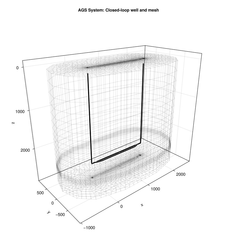

Simulate system

We set up the the simulator

sim, cfg = setup_reservoir_simulator(case;
    output_substates = true, # Store results from timesteps between
    info_level = 0, # 0=progress bar, 1=basic, 2=detailed
    initial_dt = 5.0, # Initial timestep [s]
    presolve_wells = true, # Solve wells with fixed reservoir state at the beginning of each timestep
    relaxation = true); # Enable relaxation in Newton solver

We add a specialized timestep selector to control solution quality during thermal transients. This selector monitors temperature changes and adjusts timesteps aiming at a maximum change of 5°C per timestep in both the reservoir and the well.

sel = VariableChangeTimestepSelector(:Temperature, 5.0;
    relative = false, model = :Reservoir)
push!(cfg[:timestep_selectors], sel);
sel = VariableChangeTimestepSelector(:Temperature, 5.0;
    relative = false, model = :AGS_supply)
push!(cfg[:timestep_selectors], sel);

NOTE: depending in your system, the simulation may take a few minutes to complete.

results = simulate_reservoir(case; simulator = sim, config = cfg)

ReservoirSimResult with 252 entries:

  wells (2 present):
    :AGS_supply
    :AGS_return
    Results per well:
       :lrat => Vector{Float64} of size (252,)
       :wrat => Vector{Float64} of size (252,)
       :temperature => Vector{Float64} of size (252,)
       :control => Vector{Symbol} of size (252,)
       :Aqueous_mass_rate => Vector{Float64} of size (252,)
       :bhp => Vector{Float64} of size (252,)
       :wcut => Vector{Float64} of size (252,)
       :mass_rate => Vector{Float64} of size (252,)
       :rate => Vector{Float64} of size (252,)
       :mrat => Vector{Float64} of size (252,)

  states (Vector with 252 entries, reservoir variables for each state)
    :Pressure => Vector{Float64} of size (142596,)
    :TotalMasses => Matrix{Float64} of size (1, 142596)
    :TotalThermalEnergy => Vector{Float64} of size (142596,)
    :FluidEnthalpy => Matrix{Float64} of size (1, 142596)
    :Temperature => Vector{Float64} of size (142596,)
    :PhaseMassDensities => Matrix{Float64} of size (1, 142596)
    :RockInternalEnergy => Vector{Float64} of size (142596,)
    :FluidInternalEnergy => Matrix{Float64} of size (1, 142596)

  time (report time for each state)
     Vector{Float64} of length 252

  result (extended states, reports)
     SimResult with 212 entries

  extra
     Dict{Any, Any} with keys :simulator, :config

  Completed at Apr. 01 2026 17:58 after 3 minutes, 43 seconds, 272.1 milliseconds.

Interactive Visualization

Next, we analyze and visualize the simulation results interactively to understand the AGS performance, thermal depletion patterns, and energy production characteristics throughout the 50-year operational period.

Reservoir state evolution

It is often most informative to visualize the deviation from the initial conditions to highlight the extent of the thermal depletion zones around the AGS system. We compute the change in reservoir variables to the initial state for all timesteps.

Δstates = JutulDarcy.delta_state(results.states, case.state0[:Reservoir])
plot_res_args = (
    resolution = (600, 800), aspect = :data,
    colormap = :seaborn_icefire_gradient, key = :Temperature,
    well_arg = (markersize = 0.0, ),
)
plot_reservoir(case.model, Δstates; plot_res_args...)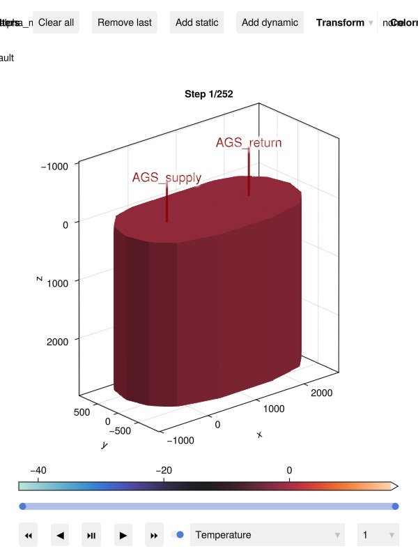

Final temperature change in the reservoir

We visualize the final temperature change in the reservoir after 50 years of operation, with a seubset of cells cut out for better visibility.

Define cells to cut out

cut_out = geo.cell_centroids[1, :] .< 750.0
cut_out = cut_out .|| geo.cell_centroids[2, :] .< 0.0
cut_out = cut_out .&& geo.cell_centroids[3, :] .< 2400

fig = Figure(size = (800, 800))
tot_time = round(sum(case.dt)/si_unit(:year), digits = 1)
ax = Axis3(fig[1, 1]; title = "Temperature after $(tot_time) years",
zreversed = true, elevation = pi/8,
aspect = :data, perspectiveness = 0.5)
plt = plot_cell_data!(ax, msh, Δstates[end][:Temperature];
    cells = .!cut_out, colormap = :seaborn_icefire_gradient)
[plot_well!(ax, msh, well;
    color = :black, markersize = 0.0, fontsize = 0.0, linewidth = 1)
    for well in values(wells)]

Colorbar(fig[2,1], plt;
    label = "ΔT (°C)", vertical = false)
fig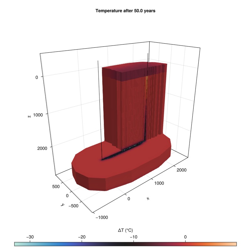

Well Performance Analysis

Examine the well responses including flow rates, pressures, and temperatures. The AGS system shows the circulation flow through the closed loop and the thermal response as the system extracts heat from the surrounding rock matrix.

plot_well_results(results.wells)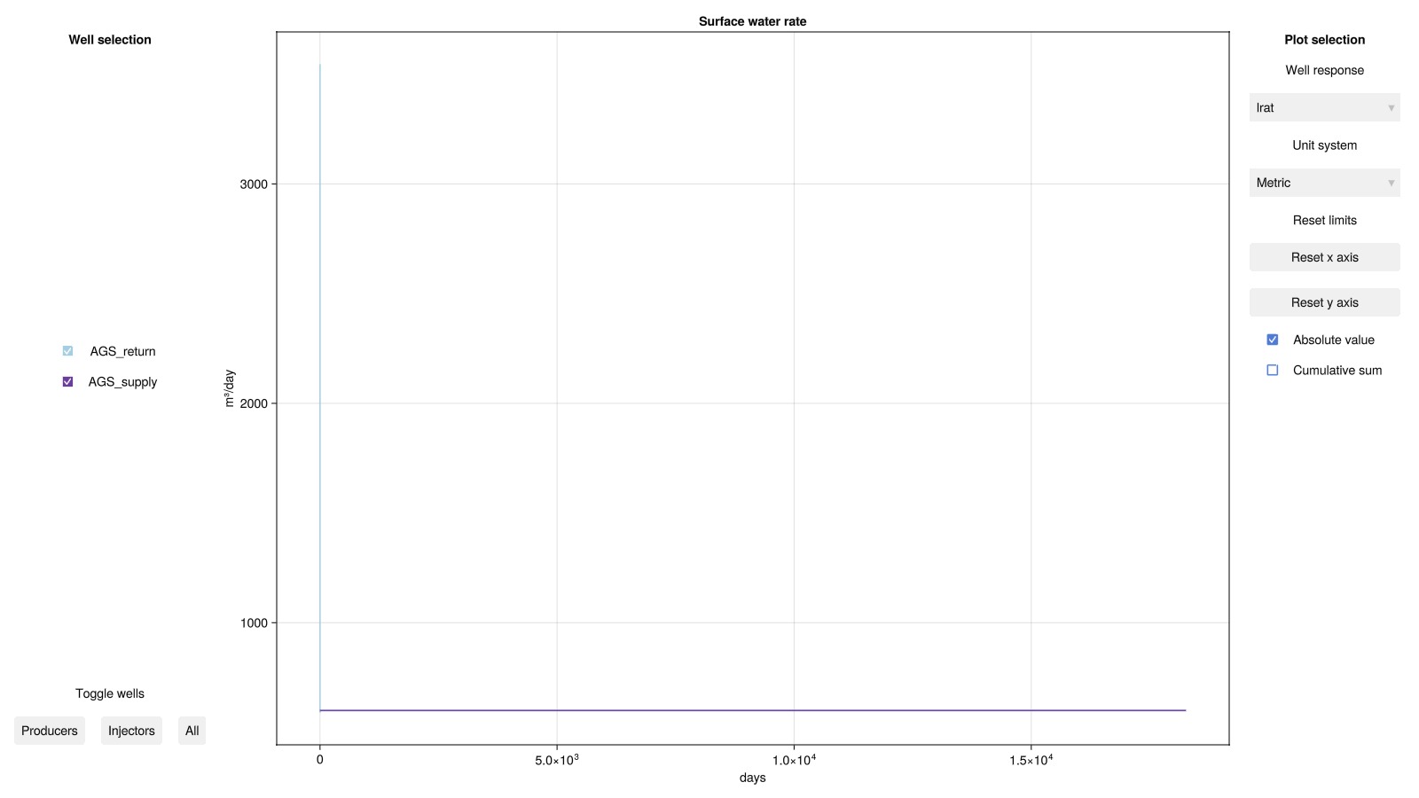

Lateral Section Analysis

We analyze the performance of the lateral sections in the AGS system by extracting temperature and power data along the lateral segments over time. This analysis helps to understand how effectively the two laterals exchange heat with the reservoir and contribute to overall energy production.

section_data = Fimbul.get_section_data_ags(
    case, results.result.states, :AGS_supply)

Dict{Any, Any} with 3 entries:
  :TotalMassFlux => [6.93199 3.46335 3.46862 6.93195; 16.3748 14.0418 14.0575 3…
  :Temperature   => [302.841 319.909 318.555 320.185; 354.865 354.865 354.865 2…
  :Power         => [1.87346e5 2.50884e5 2.31117e5 -18270.8; 1.48007e7 8.78118e…

Set up plotting utilities

colors = collect(cgrad(:BrBg, 8, categorical = true))[[2, end-1]]
function plot_lateral_data!(ax, time, data; stacked = false)
    num_laterals = size(data, 2)-2
    y_prev = zeros(size(data, 1))
    for lno = 1:num_laterals
        y = data[:, lno+1]
        if stacked
            x = vcat(time, reverse(time))
            y .+= y_prev
            y = vcat(y_prev, reverse(y))
            poly!(ax, x, y; color = colors[lno],
            strokecolor = :black, strokewidth = 1, label = "Lateral $lno")
            y_prev = data[:, lno+1]
        else
            lines!(ax, time, y; color = colors[lno], linewidth = 4, label = "Lateral $lno")
        end
    end
end

plot_lateral_data! (generic function with 1 method)

Plot lateral temperature and power over time

fig = Figure(size = (800, 800))
time = results.time ./ si_unit(:year)

ax_tmp = Axis( # Panel 1: Lateral temperature
    fig[1, 1:3]; title = "Lateral Temperature",
    ylabel = "Temperature (°C)", xlabel = "Time (years)")
T = convert_from_si.(section_data[:Temperature], :Celsius)
plot_lateral_data!(ax_tmp, time, T, stacked = false)
hidexdecorations!(ax_tmp, grid = false)

ax_pwr = Axis( # Panel 2: Lateral power
    fig[2, 1:3]; title = "Lateral Power",
    ylabel = "Power (MW)", xlabel = "Time (years)",
limits = (nothing, (-0.05, 0.5)))
MW = si_unit(:mega)*si_unit(:watt)
plot_lateral_data!(ax_pwr, time, section_data[:Power]./MW, stacked = true)

ax_lat = Axis( # Panel 3: Lateral well trajectories for reference
    fig[1:2, 4]; aspect = DataAspect(), limits = ((-150, 100), nothing),
    xticks = [-150, 100])
well_coords, _ = Fimbul.get_ags_trajectory()
for (k, wc) in enumerate(well_coords[2:3])
    lines!(ax_lat, wc[:, 2], wc[:, 1]; linewidth = 4, color = colors[k])
end

axislegend( # Add legend
    ax_tmp; position = :rt, fontsize = 20)
fig

Example on GitHub

If you would like to run this example yourself, it can be downloaded from the Fimbul.jl GitHub repository as a script.

This example took 342.098688578 seconds to complete.

---

This page was generated using Literate.jl.