Aquifer Thermal Energy Storage (ATES)

This example demonstrates comprehensive simulation and analysis of an Aquifer Thermal Energy Storage (ATES) system using Fimbul.jl. ATES systems store thermal energy by injecting hot water into subsurface aquifers during charging periods and extracting the heated water during discharge periods for heating applications.

The simulation models a two-well ATES system operating over multiple annual cycles, examining thermal efficiency, energy recovery rates, and aquifer temperature evolution. Key performance metrics include energy recovery efficiency and thermal plume propagation within the confined aquifer system.

Add required modules to namespace

using Jutul, JutulDarcy, Fimbul
using HYPRE
using Statistics
using GLMakie

Useful SI units

Kelvin, joule, watt = si_units(:Kelvin, :joule, :watt)
kilogram = si_unit(:kilogram)
meter = si_unit(:meter)
darcy = si_unit(:darcy);

Geological setup and model configuration

We first define the subsurface model with a layered aquifer system suitable for ATES operations. The model includes multiple geological layers with varying permeability and a confined aquifer target zone for thermal storage.

ATES Operational Modes:

• Charging: Inject hot water through hot well, produce through cold well

• Discharging: Produce hot water through hot well, inject cold water through cold well

• Rest: No well activity to allow thermal equilibration

The operational schedule includes charging from June to September, rest periods from October to November, and discharging from December to March. We simulate five years of operation with balanced injection/production rates to maintain stable aquifer pressure throughout the thermal storage cycles. Configure ATES system parameters and create simulation case. The system uses realistic geological and operational parameters for a medium-scale ATES installation with 400m well spacing.

num_years = 5
case = Fimbul.ates(;
    well_distance = 400.0, # Distance between wells [m]
    temperature_charge = convert_to_si(85, :Celsius),   # Hot injection temperature
    temperature_discharge = convert_to_si(20, :Celsius), # Cold injection temperature
    depths = [0.0, 850.0, 900.0, 1000.0, 1050.0, 1300.0], # Layer boundaries [m]
    porosity = [0.01, 0.05, 0.35, 0.05, 0.01], # Layer porosities [-]
    permeability = [1.0, 5.0, 1000.0, 5.0, 1.0].*1e-3.*darcy, # Layer permeabilities
    rock_thermal_conductivity = [2.5, 2.0, 1.9, 2.0, 2.5].*watt/(meter*Kelvin),
    rock_heat_capacity = 900.0*joule/(kilogram*Kelvin),   # Rock heat capacity
    aquifer_layer = 3, # Primary aquifer for thermal storage (high permeability)
    utes_schedule_args = (num_years = num_years,)
);

Inspect the ATES model

We first visualize the computational mesh, well locations, and geological structure. The mesh is strategically refined around wells and within the aquifer layer to capture thermal and hydraulic interactions accurately.

msh = physical_representation(reservoir_model(case.model).data_domain)
fig = Figure(size = (800, 800))
ax = Axis3(fig[1, 1], zreversed = true, aspect = :data,
    title = "ATES system: mesh structure and well configuration")
Jutul.plot_mesh_edges!(ax, msh, alpha = 0.2)
wells = get_model_wells(case.model)
colors = [:red, :blue]  # Hot well = red, Cold well = blue
for (i, (k, w)) in enumerate(wells)
    plot_well!(ax, msh, w, color = colors[i], linewidth = 6)
end
plot_cell_data!(ax, msh, case.input_data[:layers],
    colormap = :rainbow,
    alpha = 0.3)
fig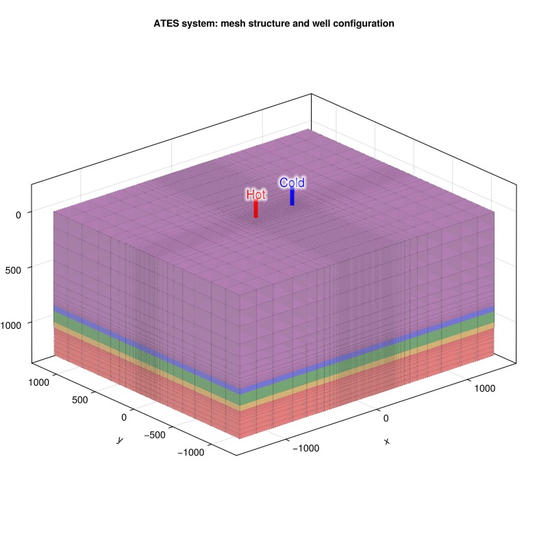

Visualize reservoir properties

Next, we examine the geological heterogeneity and porosity distribution that controls fluid flow and thermal transport within the aquifer system

plot_reservoir(case.model, key = :porosity, aspect = :data, colormap = :bilbao100)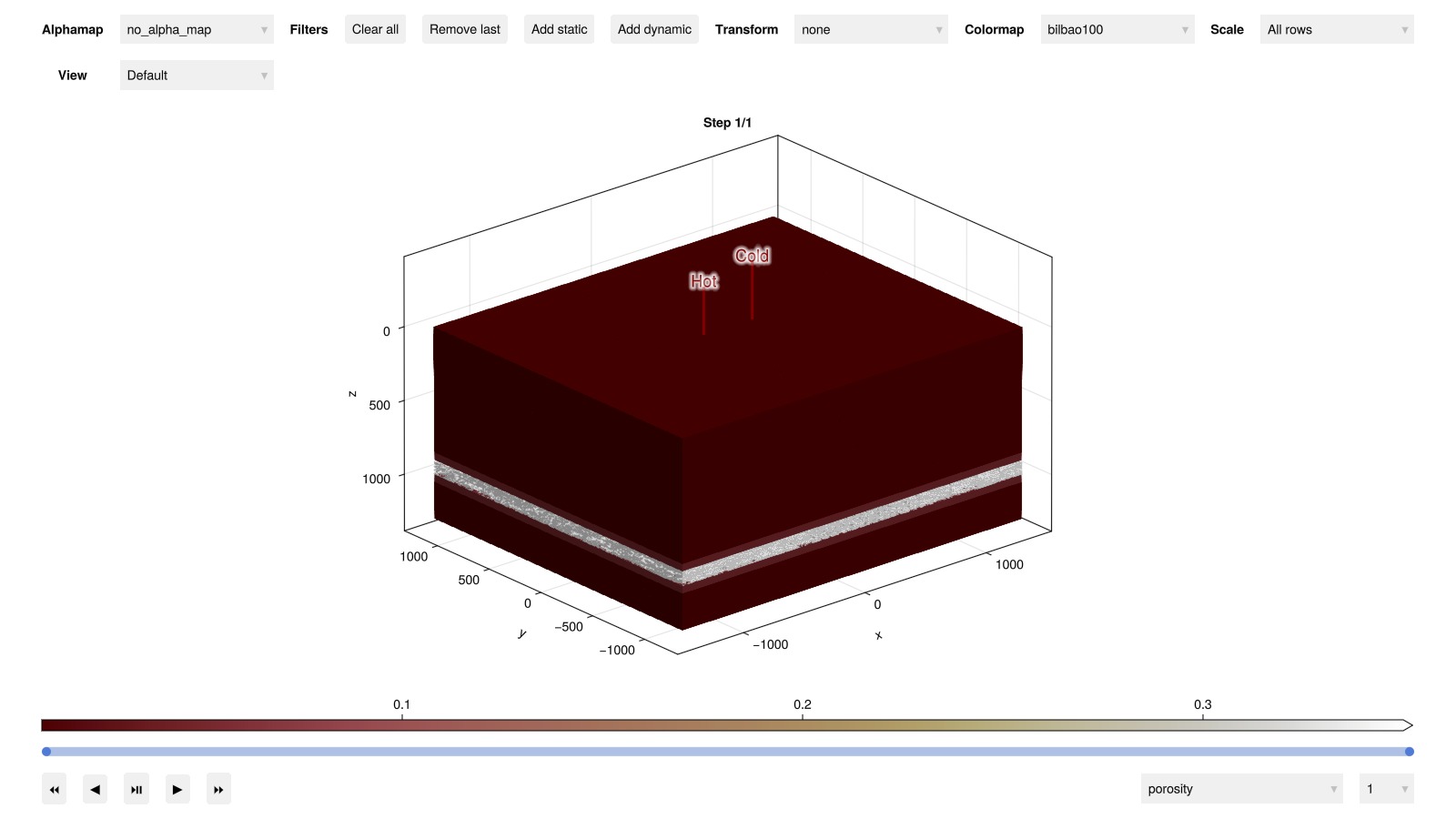

Simulate the ATES system

Transitions between injection and production modes are numerically challenging, requiring small time steps to ensure convergence and physical consistency.

sim, cfg = setup_reservoir_simulator(case; info_level = 0);
sel = JutulDarcy.ControlChangeTimestepSelector(case.model)
push!(cfg[:timestep_selectors], sel)
cfg[:timestep_max_decrease] = 1e-3; # Prevent excessive timestep reduction

Execute simulation (computation time: several minutes depending on system)

results = simulate_reservoir(case, simulator = sim, config = cfg)

ReservoirSimResult with 100 entries:

  wells (2 present):
    :Hot
    :Cold
    Results per well:
       :lrat => Vector{Float64} of size (100,)
       :wrat => Vector{Float64} of size (100,)
       :temperature => Vector{Float64} of size (100,)
       :control => Vector{Symbol} of size (100,)
       :Aqueous_mass_rate => Vector{Float64} of size (100,)
       :bhp => Vector{Float64} of size (100,)
       :wcut => Vector{Float64} of size (100,)
       :mass_rate => Vector{Float64} of size (100,)
       :rate => Vector{Float64} of size (100,)
       :mrat => Vector{Float64} of size (100,)

  states (Vector with 100 entries, reservoir variables for each state)
    :Pressure => Vector{Float64} of size (84665,)
    :TotalMasses => Matrix{Float64} of size (1, 84665)
    :TotalThermalEnergy => Vector{Float64} of size (84665,)
    :FluidEnthalpy => Matrix{Float64} of size (1, 84665)
    :Temperature => Vector{Float64} of size (84665,)
    :PhaseMassDensities => Matrix{Float64} of size (1, 84665)
    :RockInternalEnergy => Vector{Float64} of size (84665,)
    :FluidInternalEnergy => Matrix{Float64} of size (1, 84665)

  time (report time for each state)
     Vector{Float64} of length 100

  result (extended states, reports)
     SimResult with 100 entries

  extra
     Dict{Any, Any} with keys :simulator, :config

  Completed at Apr. 01 2026 18:11 after 4 minutes, 4 seconds, 464.9 milliseconds.

Visualize ATES results

We examine the temperature field evolution throughout the simulation timeline. Interactive visualization allows exploration of thermal plume development and migration patterns around the well doublet system.

plot_reservoir(case, results.states,
    key = :Temperature,
    aspect = :data,
    colormap = :seaborn_icefire_gradient)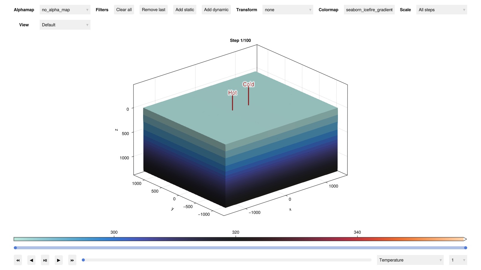

Visualize thermal plume

We plot temperature deviation from the initial state around the wells after the first and last charge and discharge stages, respectively.

Identify time steps for charge/discharge start and stop from the well controls when charging (injection) and discharging (production) phases begin and e

times = convert_from_si.(cumsum(case.dt), :year)
states = results.result.states
n_steps = length(states)
is_control = (f, ctrl) -> f[:Facility].control[:Hot] isa ctrl
ch_start = findall([true; diff([is_control(f, InjectorControl) for f in case.forces]) .> 0])
ch_stop = findall([false; diff([is_control(f, InjectorControl) for f in case.forces]) .< 0]).-1
dch_start = findall([false; diff([is_control(f, ProducerControl) for f in case.forces]) .> 0])
dch_stop = findall([false; diff([is_control(f, ProducerControl) for f in case.forces]) .< 0]).-1;

Calculate temperature changes for visualization We focus on cells in the aquifer layer that show significant temperature changes (>1°C) to visualize the thermal plume evolution during different operational phases

geo = tpfv_geometry(msh)
cell_mask = geo.cell_centroids[2,:] .> 0 .&& geo.cell_centroids[3,:] .> 900.0
T0 = case.state0[:Reservoir][:Temperature]
steps = vcat(ch_stop[1], dch_stop[1], ch_stop[end], dch_stop[end])
ΔT, cells_to_show = [], []
for (n, step) in enumerate(steps)
    ΔT_n = states[step][:Reservoir][:Temperature] .- T0
    # Only visualize cells with significant temperature change (>1°C)
    cells = cell_mask .&& abs.(ΔT_n) .> 1.0
    push!(cells_to_show, findall(cells))
    global ΔT = push!(ΔT, ΔT_n[cells])
end

Set up consistent visualization parameters for all subplots Ensures proper axis limits and color scaling across different time steps

limits = extrema(geo.cell_centroids[:, vcat(cells_to_show...)], dims=2)
Δx = [xd[2] - xd[1] for xd in limits]
limits = tuple((l .+ (-0.1*dx, 0.1*dx) for (l, dx) in zip(limits, Δx))...)
colorrange = extrema(vcat(ΔT...));

Plot temperature change after the first and last ATES operational cycles

fig = Figure(size = (1200, 600))
for (n, ΔT_n) in enumerate(ΔT)
    # Create subplot for each operational stage
    row, col = (n-1) ÷ 2 + 1, (n-1) % 2 + 1
    stage = col == 1 ? "Charge" : "Discharge"
    ax_n = Axis3(fig[row, col],
        title = "$stage, $(round(times[steps[n]], digits=1)) years",
        limits = limits, zreversed = true, azimuth = -1.1*pi/2, aspect = :data)
    # Visualize temperature changes with ice-fire colormap (blue=cold, red=hot)
    plot_cell_data!(ax_n, msh, ΔT_n,
        cells = cells_to_show[n],
        colorrange = colorrange,
        colormap = :seaborn_icefire_gradient)
    hidedecorations!(ax_n)
end

Add shared colorbar for temperature scale reference

Colorbar(fig[Int(length(steps)/2+1), 1:2],
    colormap = :seaborn_icefire_gradient,
    colorrange = colorrange,
    label = "Temperature Change (°C)",
    vertical = false)
fig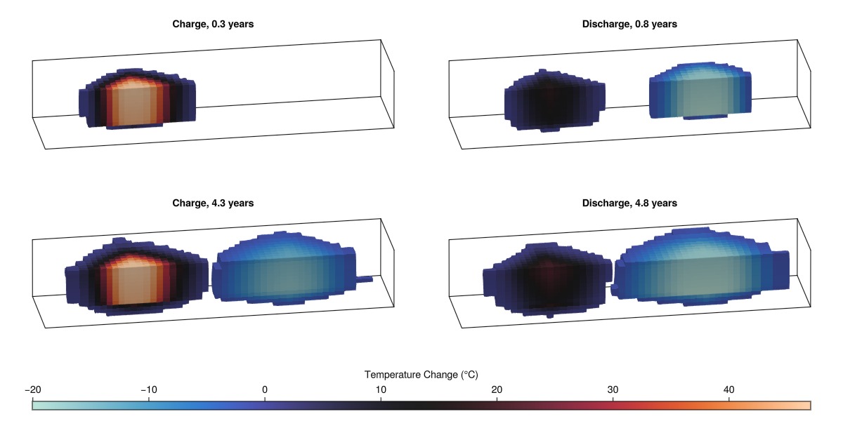

Analyze ATES performance

Examine the well responses including flow rates, pressures, and temperatures interactively to understand operational behavior

plot_well_results(results.wells)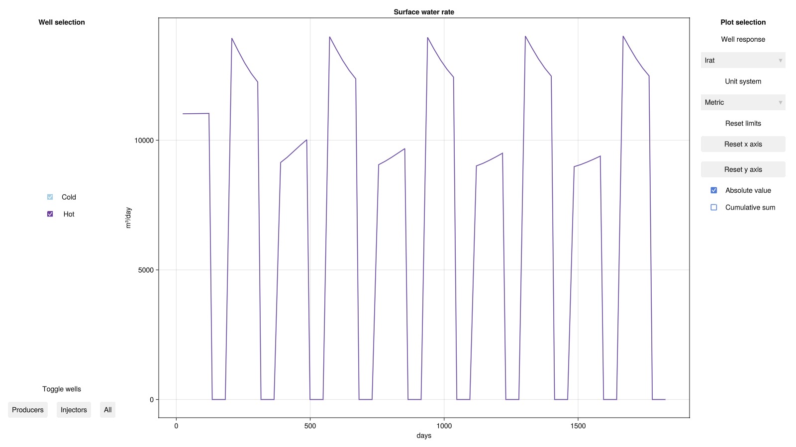

Analyze derived ATES performance metrics

We examine key performance indicators for the ATES system: flow rate, temperature, thermal effect, and energy recovery efficiency. The efficiency (recovery factor) is the most critical metric, defined as the ratio of energy extracted during discharge to energy injected during charge phases.

states = results.states;

Set up plotting utilities for performance metrics

fig_wells = Figure(size = (800, 1000))
lcolor = cgrad(:seaborn_icefire_gradient, 10, categorical = true)[8]
function make_axis(n, val, name)
    vmin, vmax = minimum(val), maximum(val)
    dv = vmax - vmin
    pad = 0.1*dv
    Axis(fig_wells[n, 1],
        xlabel = "Time (years)",
        ylabel = name,
        limits = ((times[1], times[end]), (vmin - pad, vmax + pad)),
    )
end
function plot_well_value!(ax, val, x=times)
    lines!(ax, x, val, color = lcolor, linewidth = 3)
end
function color_stages!(ax)
    ylim = ax.yaxis.attributes.limits[]
    for k in eachindex(ch_start)
        poly!(ax, [(times[ch_start[k]], ylim[1]), (times[ch_stop[k]], ylim[1]),
            (times[ch_stop[k]], ylim[2]), (times[ch_start[k]], ylim[2])],
            color = (:red, 0.1))
    end
    for k in eachindex(dch_start)
        poly!(ax, [(times[dch_start[k]], ylim[1]), (times[dch_stop[k]], ylim[1]),
            (times[dch_stop[k]], ylim[2]), (times[dch_start[k]], ylim[2])],
            color = (:blue, 0.1))
    end
end;

Plot volumetric flow rate in the hot well

rate = abs.(results.wells[:Hot][:rate]*si_unit(:hour))
ax_rate = make_axis(1, rate, "Rate (m³/h)")
plot_well_value!(ax_rate, rate)
color_stages!(ax_rate)

Plot water temperature at the hot well

temp = convert_from_si.(results.wells[:Hot][:temperature], :Celsius)
ax_temp = make_axis(2, temp, "Temperature (°C)")
plot_well_value!(ax_temp, temp)
color_stages!(ax_temp)

Plot thermal power (effect) delivered by the system

mrate = results.wells[:Hot][:mass_rate]
Cp = mean(reservoir_model(case.model).data_domain[:component_heat_capacity])
effect = mrate.*Cp.*temp
effect_mwh = abs.(effect).*1e-6  # Convert to MW
ax_effect = make_axis(3, effect_mwh, "Effect (MW)")
plot_well_value!(ax_effect, effect_mwh)
color_stages!(ax_effect)

Plot energy recovery efficiency over discharge cycles

ax_eta = make_axis(4, [-0.05,1.05], "Efficiency (–)")
energy = effect.*case.dt
for k in eachindex(ch_start)
    energy_ch = sum(energy[ch_start[k]:ch_stop[k]])
    energy_dch = abs.(cumsum(energy[dch_start[k]:dch_stop[k]]))
    η = energy_dch./energy_ch
    plot_well_value!(ax_eta, η, times[dch_start[k]:dch_stop[k]])
end
color_stages!(ax_eta)
fig_wells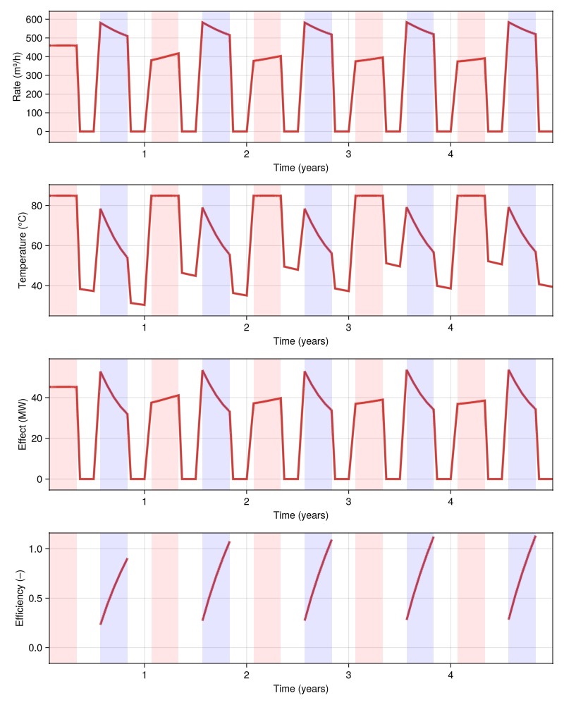

The efficiency improves with each cycle as the thermal plume matures and losses decrease, starting at approximately 81% in the first year and reaching around 89% by year five.

Aquifer temperature evolution

Examine the spatial and temporal temperature distribution in the aquifer to understand thermal plume propagation. We analyze temperature profiles along a horizontal transect between wells and track aquifer-wide temperature statistics. Notice how the hot and cold plume interactions can be seen as asymmetries in the temperature profiles around the cold well during charging and hot well during discharging.

Extract temperature along a horizontal line in the aquifer layer. This transect passes through the center of the aquifer between the two wells

layers = case.input_data[:layers]
ijk = [cell_ijk(msh, c) for c in 1:number_of_cells(msh)]
j = div(maximum(getindex.(ijk, 2)) + minimum(getindex.(ijk, 2)), 2)
k = div(maximum(getindex.(ijk[layers.==3], 3)) + minimum(getindex.(ijk[layers.==3], 3)), 2)
cells = [ix[2] == j .&& ix[3] == k for ix in ijk]
T_line = [state[:Temperature][cells] for state in results.states];

Temperature profile plotting utilities

x = geo.cell_centroids[1, cells]
function plot_aquifer_temperature!(fig, T_line, stage, cycle)
    # Create subplot for specific operational stage and cycle
    row, col = cycle, stage == "Charging" ? 1 : 2
    ax = Axis(fig[row, col],
        ylabel = "T, cycle $cycle (°C)",
        xlabel = "x (m)",
        title = cycle == 1 ? stage : "",
        limits = (nothing, (15.0, 90.0))
    )
    # Plot temperature profiles throughout the operational stage
    if stage == "Charging"
        steps = ch_start[cycle]:ch_stop[cycle]
    else
        steps = dch_start[cycle]:dch_stop[cycle]
    end
    colors = cgrad(:RdBu, length(steps), categorical = true)
    if stage == "Charging"
        colors = reverse(colors)
    end
    for (n, T_n) in enumerate(T_line[steps])
        T_n = convert_from_si.(T_n, :Celsius)
        lines!(ax, x, T_n, color = colors[n], linewidth = 3,
        label = "Year $(round(times[n], digits=1))")
    end
    return ax
end;

Plot temperature profiles during charge and discharge stages for all cycles. This shows thermal plume evolution and migration patterns over multiple years

fig = Figure(size = (800, 1000))
for cycle in 1:num_years
    # Plot charging stage temperatures (thermal plume development)
    ax_c = plot_aquifer_temperature!(fig, T_line, "Charging", cycle)
    if cycle < num_years
        hidexdecorations!(ax_c; grid=false)
    end
    # Plot discharging stage temperatures (thermal recovery and cooling)
    ax_c = plot_aquifer_temperature!(fig, T_line, "Discharging", cycle)
    if cycle < num_years
        hidedecorations!(ax_c; grid=false)
    else
        hideydecorations!(ax_c; grid=false)
    end
end
fig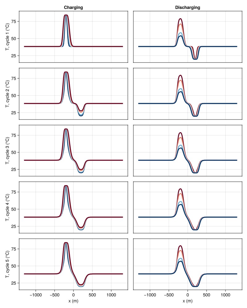

Plot aquifer temperature statistics over time

Many regions operate under legal regulations limiting the maximum allowable temperature increase in the aquifer to protect groundwater resources. This is typically defined as the mean temperature increase across the entire aquifer volume. We monitor the overall thermal state of the aquifer throughout the simulation to assess system-wide temperature impacts and thermal equilibrium.

cells = layers .== 3
T_aquifer = [state[:Temperature][cells] for state in results.states]
T_mean = [mean(convert_from_si.(T, :Celsius)) for T in T_aquifer]
fig = Figure(size = (800, 400))
ax = Axis(fig[1, 1],
    title = "Mean aquifer temperature evolution",
    xlabel = "Time (years)",
    ylabel = "Temperature (°C)",
    limits = ((times[1], times[end]), nothing),
)
lines!(ax, times, T_mean, color = lcolor, linewidth = 3)
fig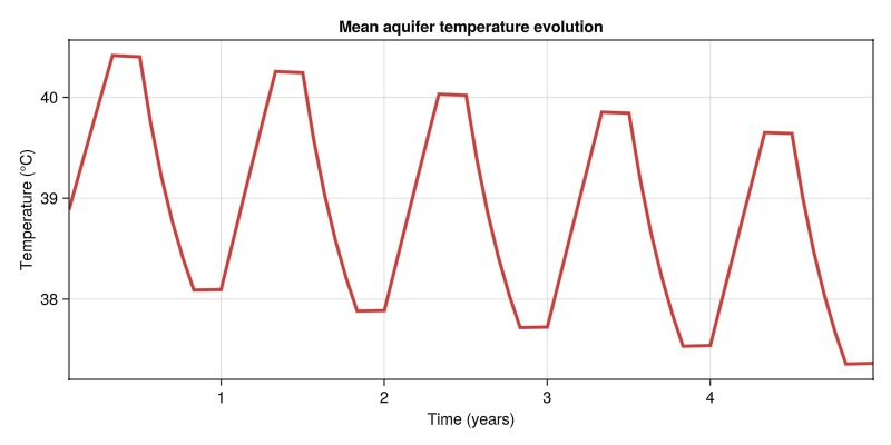

The proposed setup results in a maximum increase in the mean aquifer temperature of approximately 3.8°C due to charging. Due to a system efficiency of less than 100%, we also see a net heating effect, but this will likely stabilize over longer operational periods as thermal losses balance with recovery.

Example on GitHub

If you would like to run this example yourself, it can be downloaded from the Fimbul.jl GitHub repository as a script.

This example took 301.684135472 seconds to complete.

---

This page was generated using Literate.jl.