Digital twinning of a high-temperature aquifer thermal energy storage system
Storage ATESThe first version of this script was prepared for the 2025 DTE & AICOMAS conference:
Ø. Klemetsdal, O. Andersen, S. Krogstad, O. Møyner, "Predictive Digital Twins for Underground Thermal Energy Storage using Differentiable Programming"
The example demonstrates digital twinning of high-temperature aquifer thermal energy storage (HT-ATES). We first set up and simulate a high-fidelity model of the system, before we construct reduced-order models at a lower resolution and calibrate using adjoint-based optimization so that its output matches that of the high-fidelity model.
Add modules to namespace
using Jutul, JutulDarcy # Jutul and JutulDarcy modules
using Fimbul # Fimbul module
using HYPRE # Iterative linear solvers
using GLMakie # Visualization
Set up model
We use the first realization of the EGG benchmark model [2], and place a well doublet near the center of the domain. The fluid model is a single-phase water system with PVT formulations taken from the NIST database, which can be conveniently set up with the :geothermal keyword.
The HT-ATES system is operated by charging the aquifer through the main well (labelled "Hot" in this setup) with water at 25 l/s and 90°C from June to September while a supporting well (labelled "Cold") is used to extract water at a constant BHP of 25 bar. The system is then discharged from December to March by producing hot water from the main well at a rate of 25 l/s with the supporting well injecting water at 10°C at a BHP of 45 bar. For the remaining months, the system is left to rest with no external forces applied. This cycle of charge – rest – discharge – rest is repeated for a total of 5 years.
hifi = egg_ates(; use_bc = false, num_reports = 12)Jutul case with 240 time-steps (4 years, 52 weeks, 1.03 day) and forces for each step.
Model:
MultiModel with 5 models and 24 cross-terms. 37181 equations, 37181 degrees of freedom and 301553 parameters.
models:
1) Reservoir (37106x37106)
SinglePhaseSystem{AqueousPhase, Tuple{Float64}}(AqueousPhase(), (998.20715,))
∈ MinimalTPFATopology (18553 cells, 52113 faces)
2) WellA (20x20)
SinglePhaseSystem{AqueousPhase, Tuple{Float64}}(AqueousPhase(), (998.20715,))
∈ MultiSegmentWell [WellA] (7 nodes, 6 segments, 7 perforations)
3) WellB (20x20)
SinglePhaseSystem{AqueousPhase, Tuple{Float64}}(AqueousPhase(), (998.20715,))
∈ MultiSegmentWell [WellB] (7 nodes, 6 segments, 7 perforations)
4) WellObs (20x20)
SinglePhaseSystem{AqueousPhase, Tuple{Float64}}(AqueousPhase(), (998.20715,))
∈ MultiSegmentWell [WellObs] (7 nodes, 6 segments, 7 perforations)
5) Facility (15x15)
JutulDarcy.FacilitySystem{SinglePhaseSystem{AqueousPhase, Tuple{Float64}}}(SinglePhaseSystem{AqueousPhase, Tuple{Float64}}(AqueousPhase(), (998.20715,)))
∈ WellGroup([:WellA, :WellB, :WellObs], true, true)
cross_terms:
1) WellA <-> Reservoir (Eqs: mass_conservation <-> mass_conservation)
JutulDarcy.ReservoirFromWellFlowCT
2) WellA <-> Reservoir (Eqs: energy_conservation <-> energy_conservation)
JutulDarcy.ReservoirFromWellThermalCT
3) WellB <-> Reservoir (Eqs: mass_conservation <-> mass_conservation)
JutulDarcy.ReservoirFromWellFlowCT
4) WellB <-> Reservoir (Eqs: energy_conservation <-> energy_conservation)
JutulDarcy.ReservoirFromWellThermalCT
5) WellObs <-> Reservoir (Eqs: mass_conservation <-> mass_conservation)
JutulDarcy.ReservoirFromWellFlowCT
6) WellObs <-> Reservoir (Eqs: energy_conservation <-> energy_conservation)
JutulDarcy.ReservoirFromWellThermalCT
7) Facility -> WellA (Eq: mass_conservation)
JutulDarcy.WellFromFacilityFlowCT
8) WellA -> Facility (Eq: bottom_hole_pressure_equation)
JutulDarcy.FacilityFromWellBottomHolePressureCT
9) WellA -> Facility (Eq: surface_phase_rates_equation)
JutulDarcy.FacilityFromSurfacePhaseRatesCT
10) Facility -> WellA (Eq: energy_conservation)
JutulDarcy.WellFromFacilityThermalCT
11) WellA -> Facility (Eq: temperature_equation)
JutulDarcy.FacilityFromWellTemperatureCT
12) WellA -> Facility (Eq: enthalpy_equation)
JutulDarcy.FacilityFromWellEnthalpyCT
13) Facility -> WellB (Eq: mass_conservation)
JutulDarcy.WellFromFacilityFlowCT
14) WellB -> Facility (Eq: bottom_hole_pressure_equation)
JutulDarcy.FacilityFromWellBottomHolePressureCT
15) WellB -> Facility (Eq: surface_phase_rates_equation)
JutulDarcy.FacilityFromSurfacePhaseRatesCT
16) Facility -> WellB (Eq: energy_conservation)
JutulDarcy.WellFromFacilityThermalCT
17) WellB -> Facility (Eq: temperature_equation)
JutulDarcy.FacilityFromWellTemperatureCT
18) WellB -> Facility (Eq: enthalpy_equation)
JutulDarcy.FacilityFromWellEnthalpyCT
19) Facility -> WellObs (Eq: mass_conservation)
JutulDarcy.WellFromFacilityFlowCT
20) WellObs -> Facility (Eq: bottom_hole_pressure_equation)
JutulDarcy.FacilityFromWellBottomHolePressureCT
21) WellObs -> Facility (Eq: surface_phase_rates_equation)
JutulDarcy.FacilityFromSurfacePhaseRatesCT
22) Facility -> WellObs (Eq: energy_conservation)
JutulDarcy.WellFromFacilityThermalCT
23) WellObs -> Facility (Eq: temperature_equation)
JutulDarcy.FacilityFromWellTemperatureCT
24) WellObs -> Facility (Eq: enthalpy_equation)
JutulDarcy.FacilityFromWellEnthalpyCT
Model storage will be optimized for runtime performance.Visualize the model
We visualize the model interactively using plot_reservoir.
plot_reservoir(hifi, reservoir_model(hifi.model).data_domain)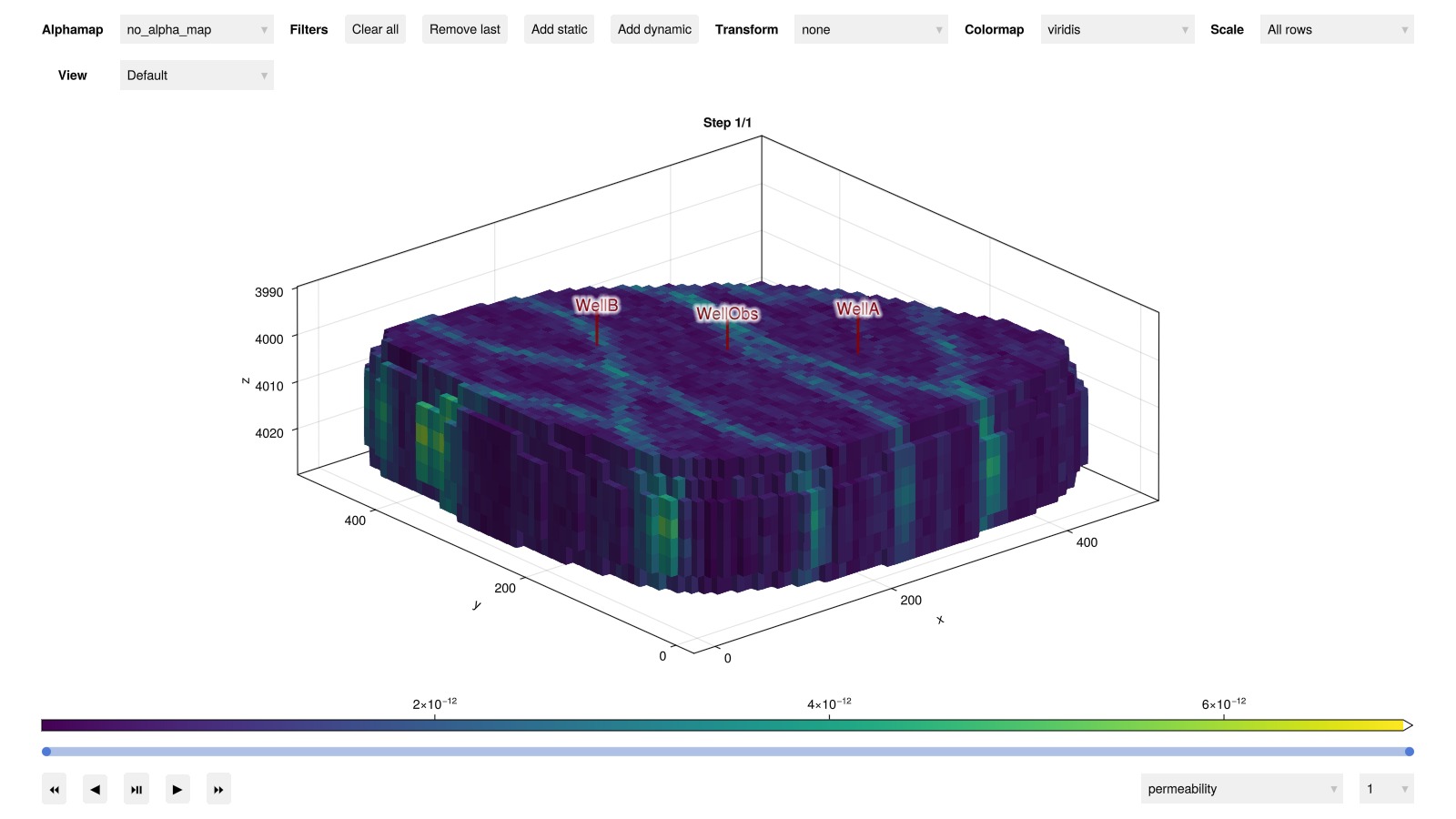
Simulate high-fidelity model
We set up a simulator for the high-fidelity model and simulate the system.
results_hifi = simulate_reservoir(hifi)ReservoirSimResult with 240 entries:
wells (3 present):
:WellObs
:WellB
:WellA
Results per well:
:lrat => Vector{Float64} of size (240,)
:wrat => Vector{Float64} of size (240,)
:temperature => Vector{Float64} of size (240,)
:control => Vector{Symbol} of size (240,)
:Aqueous_mass_rate => Vector{Float64} of size (240,)
:bhp => Vector{Float64} of size (240,)
:wcut => Vector{Float64} of size (240,)
:mass_rate => Vector{Float64} of size (240,)
:rate => Vector{Float64} of size (240,)
:mrat => Vector{Float64} of size (240,)
states (Vector with 240 entries, reservoir variables for each state)
:Pressure => Vector{Float64} of size (18553,)
:TotalMasses => Matrix{Float64} of size (1, 18553)
:TotalThermalEnergy => Vector{Float64} of size (18553,)
:FluidEnthalpy => Matrix{Float64} of size (1, 18553)
:Temperature => Vector{Float64} of size (18553,)
:PhaseMassDensities => Matrix{Float64} of size (1, 18553)
:RockInternalEnergy => Vector{Float64} of size (18553,)
:FluidInternalEnergy => Matrix{Float64} of size (1, 18553)
:PhaseViscosities => Matrix{Float64} of size (1, 18553)
time (report time for each state)
Vector{Float64} of length 240
result (extended states, reports)
SimResult with 240 entries
extra
Dict{Any, Any} with keys :simulator, :config
Completed at Jun. 20 2026 07:43 after 47 seconds, 61 milliseconds, 659 microseconds.Visualize the reservoir states
We visualize the results of the high-fidelity simulation interactively using plot_reservoir. We see that a hot thermal plume develops around the main well, while a cold plume develops around the supporting well. After a few cycles, the plumes start to interact slightly.
plot_reservoir(hifi, results_hifi.states;
    key = :Temperature, step = length(hifi.dt),
    colormap = :seaborn_icefire_gradient)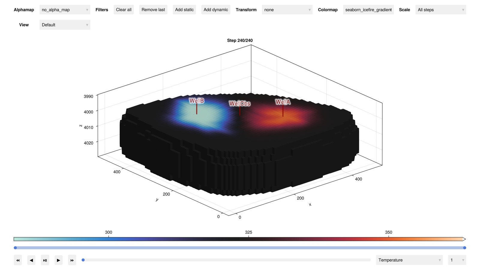
Inspect well output
We can also inspect the well output using plot_well_results.
plot_well_results(results_hifi.wells)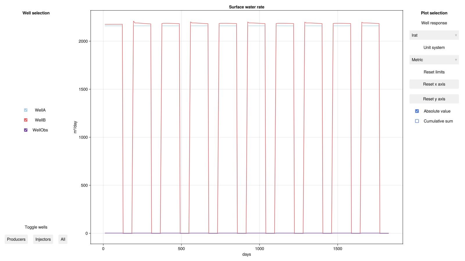
Construct proxy model
The high-fidelity model is posed on a logically Cartesian mesh with 60×60×7 cells. We construct a proxy model by coarsening the high-fidelity model to 15×15×3 cells using the coarsen_reservoir_case function.
coarsening = (15,15,3)
proxy = JutulDarcy.coarsen_reservoir_case(hifi, coarsening,
    method=:ijk,
    setup_arg = (block_backend = true,);
)
results_proxy = simulate_reservoir(proxy, info_level=0)
plot_reservoir(proxy, results_proxy.states;
    key = :Temperature, step = length(hifi.dt),
    colormap = :seaborn_icefire_gradient)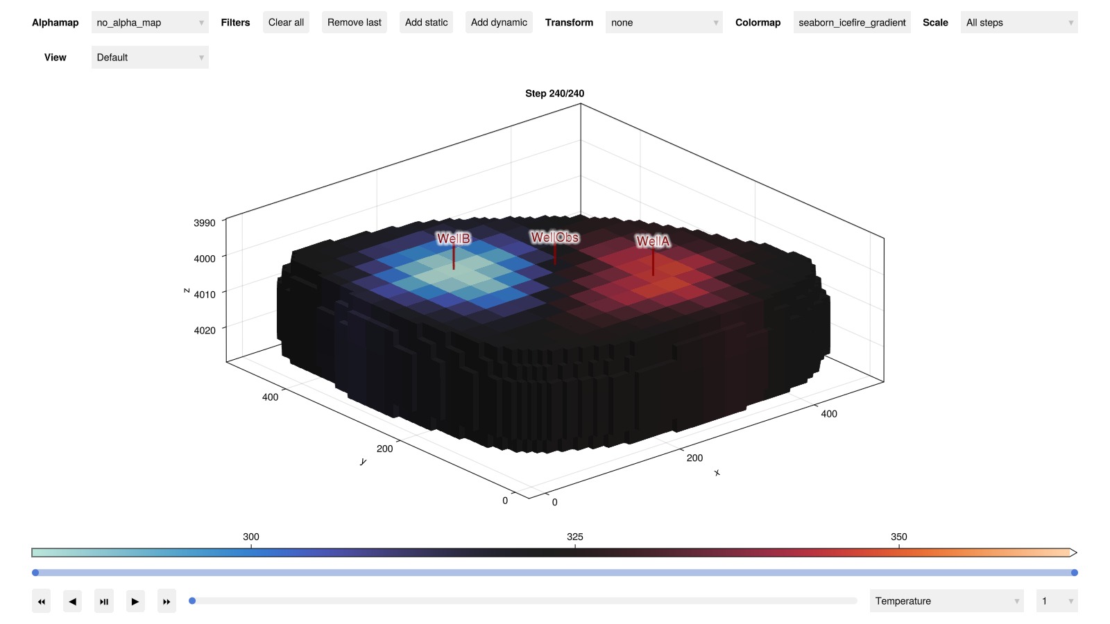
Compare proxy models to high-fidelity model
We compare the well output of the proxy models to the high-fidelity model.
plot_well_results([results_hifi.wells, results_proxy.wells],
    names = ["High-fidelity", "Proxy"])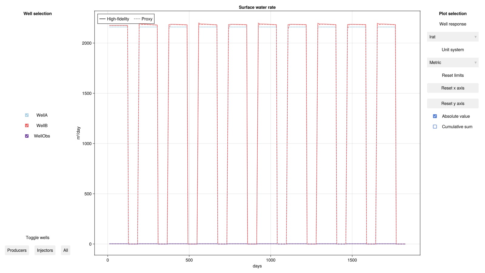
Define mismatch objective function
We define an objective function that measures the mismatch in well output between the high-fidelity model and the proxy model. The objective function is defined as the sum of the squared differences in production temperature of all wells, weighted by the inverse of the units of the respective quantities. The objective function is also scaled by the total time simulated in the high-fidelity model.
states_hf = results_hifi.result.states
states_proxy = results_proxy.result.states;
We calibrate against the first two years. Since we have defined report steps of 1/4 month, this corresponds to the first 12_4_2 steps. To see the effect of more or less data used for calibration, and to exclude/include data from one or more of the wells and WellObs, you can change num_years_cal and wells_cal below.
num_years_cal = 2
n_steps = 12*4*num_years_cal
wells_cal = [:WellA, :WellB]
objective = (model, state, dt, step_no, forces) ->
    well_mismatch_thermal(model, wells_cal,
        states_hf, state, dt, step_no, forces;
        scale=sum(hifi.dt[1:n_steps]),
        w_bhp = 0.0,
        w_temp = 1.0/si_unit(:Kelvin),
        w_energy = 0.0,
    );
Compute mismatch for initial proxy model
obj0 = Jutul.evaluate_objective(
    objective, proxy.model, states_proxy[1:n_steps],
    proxy.dt[1:n_steps], proxy.forces[1:n_steps])
println("Initial proxy mismatch: $obj0")
Initial proxy mismatch: 13.528603254598382Set up optimization
We use setup_reservoir_dict_optimization to create a dict-based optimization setup for the calibration period of the proxy model.
dprm = setup_reservoir_dict_optimization(deepcopy(proxy[1:n_steps]));Declare free parameters and bounds
We declare the subset of parameters to calibrate together with their relative bounds. Parameters that are not freed here remain fixed.
free_optimization_parameter!( # Permeability
    dprm, [:model, :permeability]; rel_min = 1e-6, rel_max = 1e1)
free_optimization_parameter!( # Porosity
    dprm, [:model, :porosity]; abs_min = 0.0001, abs_max = 0.9)
free_optimization_parameter!( # Rock density
    dprm, [:model, :rock_density]; abs_min = 100.0, abs_max = 4000.0)
free_optimization_parameter!( # Rock heat capacity
    dprm, [:model, :rock_heat_capacity]; abs_min = 100.0, abs_max = 2000.0)
free_optimization_parameter!( # Rock thermal conductivity
    dprm, [:model, :rock_thermal_conductivity]; rel_min = 1e-6, rel_max = 1e1)
free_optimization_parameter!( # Fluid thermal conductivity
    dprm, [:model, :fluid_thermal_conductivity]; rel_min = 1e-6, rel_max = 1e1)
DictParameters with 16 parameters (6 active), and 0 multipliers:
Active optimization parameters
┌──────────────────────────────────┬─────────────────────┬───────┬──────────┬───
│ Name │ Initial value │ Count │ Min │ ⋯
├──────────────────────────────────┼─────────────────────┼───────┼──────────┼───
│ model.permeability │ 5.55e-13 ± 3.09e-12 │ 1683 │ 2.94e-20 │ ⋯
│ model.porosity │ 0.2 ± 2.5e-16 │ 561 │ 0.0001 │ ⋯
│ model.rock_density │ 2000.0 ± 0.0 │ 561 │ 100.0 │ ⋯
│ model.rock_heat_capacity │ 900.0 ± 0.0 │ 561 │ 100.0 │ ⋯
│ model.rock_thermal_conductivity │ 3.0 ± 0.0 │ 561 │ 3.0e-6 │ ⋯
│ model.fluid_thermal_conductivity │ 0.598 ± 3.33e-16 │ 561 │ 5.98e-7 │ ⋯
└──────────────────────────────────┴─────────────────────┴───────┴──────────┴───
1 column omitted
Inactive optimization parameters
┌──────────────────────────────────┬──────────────────────────────┬───────┬─────
│ Name │ Initial value │ Count │ Mi ⋯
├──────────────────────────────────┼──────────────────────────────┼───────┼─────
│ model.component_heat_capacity │ 4180.0 ± 0.0 │ 561 │ ⋯
│ model.net_to_gross │ 1.0 ± 0.0 │ 561 │ ⋯
│ wells.WellA.WellIndices │ 1.04e-11, 6.09e-12, 6.85e-12 │ 3 │ ⋯
│ wells.WellA.WellIndicesThermal │ 39.2, 26.2, 26.2 │ 3 │ ⋯
│ wells.WellB.WellIndices │ 1.49e-11, 1.06e-11, 9.99e-12 │ 3 │ ⋯
│ wells.WellB.WellIndicesThermal │ 39.2, 26.2, 26.2 │ 3 │ ⋯
│ wells.WellObs.WellIndices │ 1.12e-11, 7.2e-12, 6.89e-12 │ 3 │ ⋯
│ wells.WellObs.WellIndicesThermal │ 39.2, 26.2, 26.2 │ 3 │ ⋯
│ state0.Pressure │ 5.13e6 ± 92100.0 │ 561 │ ⋯
│ state0.Temperature │ 324.0 ± 0.282 │ 561 │ ⋯
└──────────────────────────────────┴──────────────────────────────┴───────┴─────
2 columns omitted
No multipliers set.Calibrate proxy model
We run the optimization using the built-in L-BFGS optimizer.
prm_opt = optimize_reservoir(dprm, objective;
    simulator_arg=(output_substates=false,), gradient_scaling=false, max_it=200)
OrderedDict{Symbol, Any} with 4 entries:
:model => OrderedDict{Symbol, Any}(:component_heat_capacity=>[4184.0, 41…
:parameters => OrderedDict{Symbol, Any}()
:wells => OrderedDict{Symbol, Any}(:WellA=>OrderedDict{Symbol, Any}(:Wel…
:state0 => OrderedDict{Symbol, Any}(:Pressure=>[5.06093e6, 5.04616e6, 5.0…Reconstruct full-schedule case from calibrated parameters
The optimization was posed on the calibration period only. We now apply the optimized parameters to the full five-year schedule for prediction.
case_opt = dprm.setup_function(prm_opt)
proxy_cal = JutulCase(case_opt.model, proxy.dt, proxy.forces;
    state0 = proxy.state0, parameters = case_opt.parameters)
Jutul case with 240 time-steps (4 years, 52 weeks, 1.03 day) and forces for each step.
Model:
MultiModel with 5 models and 24 cross-terms. 1170 equations, 1170 degrees of freedom and 8603 parameters.
models:
1) Reservoir (1122x1122)
SinglePhaseSystem{AqueousPhase, Tuple{Float64}}(AqueousPhase(), (998.20715,))
∈ MinimalTPFATopology (561 cells, 1406 faces)
2) WellA (11x11)
SinglePhaseSystem{AqueousPhase, Tuple{Float64}}(AqueousPhase(), (998.20715,))
∈ MultiSegmentWell [WellA] (4 nodes, 3 segments, 3 perforations)
3) WellB (11x11)
SinglePhaseSystem{AqueousPhase, Tuple{Float64}}(AqueousPhase(), (998.20715,))
∈ MultiSegmentWell [WellB] (4 nodes, 3 segments, 3 perforations)
4) WellObs (11x11)
SinglePhaseSystem{AqueousPhase, Tuple{Float64}}(AqueousPhase(), (998.20715,))
∈ MultiSegmentWell [WellObs] (4 nodes, 3 segments, 3 perforations)
5) Facility (15x15)
JutulDarcy.FacilitySystem{SinglePhaseSystem{AqueousPhase, Tuple{Float64}}}(SinglePhaseSystem{AqueousPhase, Tuple{Float64}}(AqueousPhase(), (998.20715,)))
∈ WellGroup([:WellA, :WellB, :WellObs], true, true)
cross_terms:
1) WellA <-> Reservoir (Eqs: mass_conservation <-> mass_conservation)
JutulDarcy.ReservoirFromWellFlowCT
2) WellA <-> Reservoir (Eqs: energy_conservation <-> energy_conservation)
JutulDarcy.ReservoirFromWellThermalCT
3) WellB <-> Reservoir (Eqs: mass_conservation <-> mass_conservation)
JutulDarcy.ReservoirFromWellFlowCT
4) WellB <-> Reservoir (Eqs: energy_conservation <-> energy_conservation)
JutulDarcy.ReservoirFromWellThermalCT
5) WellObs <-> Reservoir (Eqs: mass_conservation <-> mass_conservation)
JutulDarcy.ReservoirFromWellFlowCT
6) WellObs <-> Reservoir (Eqs: energy_conservation <-> energy_conservation)
JutulDarcy.ReservoirFromWellThermalCT
7) Facility -> WellA (Eq: mass_conservation)
JutulDarcy.WellFromFacilityFlowCT
8) WellA -> Facility (Eq: bottom_hole_pressure_equation)
JutulDarcy.FacilityFromWellBottomHolePressureCT
9) WellA -> Facility (Eq: surface_phase_rates_equation)
JutulDarcy.FacilityFromSurfacePhaseRatesCT
10) Facility -> WellA (Eq: energy_conservation)
JutulDarcy.WellFromFacilityThermalCT
11) WellA -> Facility (Eq: temperature_equation)
JutulDarcy.FacilityFromWellTemperatureCT
12) WellA -> Facility (Eq: enthalpy_equation)
JutulDarcy.FacilityFromWellEnthalpyCT
13) Facility -> WellB (Eq: mass_conservation)
JutulDarcy.WellFromFacilityFlowCT
14) WellB -> Facility (Eq: bottom_hole_pressure_equation)
JutulDarcy.FacilityFromWellBottomHolePressureCT
15) WellB -> Facility (Eq: surface_phase_rates_equation)
JutulDarcy.FacilityFromSurfacePhaseRatesCT
16) Facility -> WellB (Eq: energy_conservation)
JutulDarcy.WellFromFacilityThermalCT
17) WellB -> Facility (Eq: temperature_equation)
JutulDarcy.FacilityFromWellTemperatureCT
18) WellB -> Facility (Eq: enthalpy_equation)
JutulDarcy.FacilityFromWellEnthalpyCT
19) Facility -> WellObs (Eq: mass_conservation)
JutulDarcy.WellFromFacilityFlowCT
20) WellObs -> Facility (Eq: bottom_hole_pressure_equation)
JutulDarcy.FacilityFromWellBottomHolePressureCT
21) WellObs -> Facility (Eq: surface_phase_rates_equation)
JutulDarcy.FacilityFromSurfacePhaseRatesCT
22) Facility -> WellObs (Eq: energy_conservation)
JutulDarcy.WellFromFacilityThermalCT
23) WellObs -> Facility (Eq: temperature_equation)
JutulDarcy.FacilityFromWellTemperatureCT
24) WellObs -> Facility (Eq: enthalpy_equation)
JutulDarcy.FacilityFromWellEnthalpyCT
Model storage will be optimized for runtime performance.Simulate the full schedule using the calibrated proxy
results_proxy_cal = simulate_reservoir(proxy_cal)
states_proxy_cal = results_proxy_cal.result.states
obj = Jutul.evaluate_objective(
    objective, proxy_cal.model, states_proxy_cal[1:n_steps],
    proxy_cal.dt[1:n_steps], proxy_cal.forces[1:n_steps])
println("Final proxy mismatch: $obj")
Jutul: Simulating 4 years, 52.15 weeks as 240 report steps
╭────────────────┬───────────┬───────────────┬────────────╮
│ Iteration type │ Avg/step │ Avg/ministep │ Total │
│ │ 240 steps │ 251 ministeps │ (wasted) │
├────────────────┼───────────┼───────────────┼────────────┤
│ Newton │ 2.48333 │ 2.3745 │ 596 (15) │
│ Linearization │ 3.52917 │ 3.3745 │ 847 (16) │
│ Linear solver │ 9.59167 │ 9.17131 │ 2302 (91) │
│ Precond apply │ 19.1833 │ 18.3426 │ 4604 (182) │
╰────────────────┴───────────┴───────────────┴────────────╯
╭───────────────┬────────┬────────────┬────────╮
│ Timing type │ Each │ Relative │ Total │
│ │ ms │ Percentage │ s │
├───────────────┼────────┼────────────┼────────┤
│ Properties │ 0.1041 │ 3.52 % │ 0.0620 │
│ Equations │ 0.3719 │ 17.89 % │ 0.3150 │
│ Assembly │ 0.2334 │ 11.22 % │ 0.1977 │
│ Linear solve │ 0.1425 │ 4.82 % │ 0.0849 │
│ Linear setup │ 0.9283 │ 31.41 % │ 0.5533 │
│ Precond apply │ 0.0598 │ 15.62 % │ 0.2752 │
│ Update │ 0.0852 │ 2.88 % │ 0.0508 │
│ Convergence │ 0.1782 │ 8.57 % │ 0.1509 │
│ Input/Output │ 0.0357 │ 0.51 % │ 0.0090 │
│ Other │ 0.1050 │ 3.55 % │ 0.0626 │
├───────────────┼────────┼────────────┼────────┤
│ Total │ 2.9552 │ 100.00 % │ 1.7613 │
╰───────────────┴────────┴────────────┴────────╯
Final proxy mismatch: 5.184456593933642Plot the calibrated results
Finally, we plot the resulting production temperatures for the high-fidelity and proxy model. The calibrated proxy does a good job of reproducing the temperatures used for calibration, but the prediction for the remaining three years of storage are not perfect, with the calibrated proxy model showing mismatch comparable to the initial proxy model for WellA and WellB in the final year.
fig = Figure(size = (800, 1200), fontsize = 20)
time_tot = results_hifi.wells.time/si_unit(:year)
for (wno, well) in enumerate(well_symbols(hifi.model))
    ax = Axis(fig[wno, 1], xlabel = "Time (years)", ylabel = "Temperature (°C)",
        title = "Well: $well")
    plot_well_data!(ax, time_tot, states_hf,
        vcat([states_proxy], [states_proxy_cal], [states_proxy_cal]);
        wells = [well],
        field = :Temperature,
        nan_ix = [
            missing,
            n_steps+1:length(hifi.dt),
            1:n_steps-1],
        names=vcat(
            "High-fidelity",
            "Proxy (initial)",
            "Proxy (calibration)",
            "Proxy (prediction)"),
        legend = wno == 2
        )
end
fig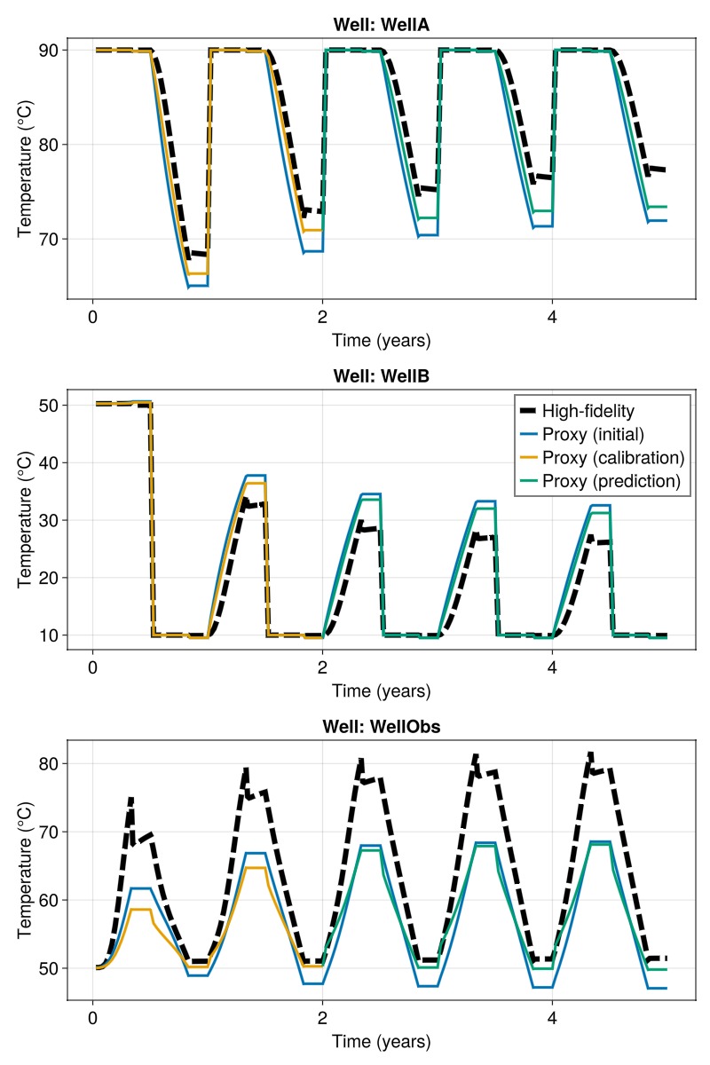
Example on GitHub
If you would like to run this example yourself, it can be downloaded from the Fimbul.jl GitHub repository as a script.
This example took 260.600826859 seconds to complete.This page was generated using Literate.jl.