Heat equation in 1D

This example demonstrates the classical solution of the heat equation in 1D and compares the analytical solution to the numerical solution obtained using JutulDarcy to verify the accuracy and convergence properties of the numerical scheme.

Add required modules and define convenience functions for unit conversion

using Jutul, JutulDarcy, Fimbul
using LinearAlgebra
using HYPRE
using GLMakie

to_kelvin = T -> convert_to_si(T, :Celsius)
to_celsius = T -> convert_from_si(T, :Celsius)

#3 (generic function with 1 method)

The 1D heat equation

We consider a piece of solid rock with length $L$ and constant thermal conductivity $\lambda$, heat capacity $C_p$ and density $\rho$. Conservation of energy in this system takes the form of the archetypical heat equation:

$\dot{T}=\alpha \mathrm{\Delta }T$, $\alpha =\frac{\lambda }{\rho C_p}$

where $T$ is the temperature and $\alpha$ is the thermal diffusivity. For this problem, we impose fixed boundary conditions $T(0,t)=T(L,t)=T_b$ and initial conditions $T(x,0)=T_0(x)$. The analytical solution to this boundary value problem can be found in any textbook on partial differential equations, and is given by the Fourier series:

$T(x,t)=T_b+\sum _{k=1}^{\mathrm{\infty }}{C}_k\exp (-\alpha (\frac{k\pi }{L}{)}^{2}t)\sin (\frac{k\pi }{L}x)$

where the Fourier coefficients $C_k$ are determined by the initial condition and boundary conditions through the orthogonality of sine functions:

$C_k=\frac{2}{L}{\int }_0^L(T_0(x)-T_b)\sin (\frac{n\pi }{L}x)dx$

Simple initial conditions

We first consider a simple initial condition where the initial temperature profile takes the form of a sine curve,

$T_0(x)=T_{max}\sin (\frac{\pi }{L}x)$

L = 100.0
T_b = to_kelvin(10.0)
T_0 = x -> to_kelvin(90.0) .* sin(π * x / L) .+ T_b;
case, sol, x, t = analytical_1d(
    L=L, temperature_boundary=T_b, initial_condition=T_0,
    num_cells=100, num_steps=100);

results = simulate_reservoir(case, info_level=0)

ReservoirSimResult with 100 entries:

  wells (0 present):

  states (Vector with 100 entries, reservoir variables for each state)
    :Pressure => Vector{Float64} of size (100,)
    :TotalMasses => Matrix{Float64} of size (1, 100)
    :TotalThermalEnergy => Vector{Float64} of size (100,)
    :FluidEnthalpy => Matrix{Float64} of size (1, 100)
    :Temperature => Vector{Float64} of size (100,)

  time (report time for each state)
     Vector{Float64} of length 100

  result (extended states, reports)
     SimResult with 100 entries

  extra
     Dict{Any, Any} with keys :simulator, :config

  Completed at Jul. 07 2025 22:07 after 10 seconds, 35 milliseconds, 170.8 microseconds.

Visualize temperature evolution

We set up a visualization function that plots both numerical and analytical temperature profiles at selected timesteps. This allows us to visually assess the agreement between the two solutions as thermal diffusion progresses.

function plot_temperature_1d(case, sol_n, sol_a, x_n, t_n, n)
    fig = Figure(size=(800, 600), fontsize=20)
    ax = Axis(fig[1, 1]; xlabel="Distance (m)", ylabel="Temperature (°C)")

    x_a = range(0, 100, length=500)

    N = length(t_n)
    α = (N^(1 / (n - 1)) - 1)
    timesteps = Int.(round.((1 + α) .^ (1:n-1)))
    pushfirst!(timesteps, 0) # Add initial time

    colors = cgrad(:Spectral, n, categorical=true)
    for (i, k) = enumerate(timesteps)
        if k == 0
            T_n = to_celsius.(case.state0[:Reservoir][:Temperature])
            lines!(ax, x_n, T_n, linestyle=(:dash, 1), linewidth=6,
                color=colors[i], label="Analytical")
            lines!(ax, x_n, T_n, linewidth=2, color=colors[i], label="Numerical")
        else
            T_a = to_celsius.(sol_a(x_a, t_n[k]))
            T_n = to_celsius.(sol_n.states[k][:Temperature])
            lines!(ax, x_a, T_a, linestyle=(:dash, 1), linewidth=6,
                color=colors[i])
            lines!(ax, x_n, T_n, linewidth=2, color=colors[i])
        end
    end
    Legend(fig[1, 2], ax)
    fig
end

plot_temperature_1d(case, results, sol, x, t, 10)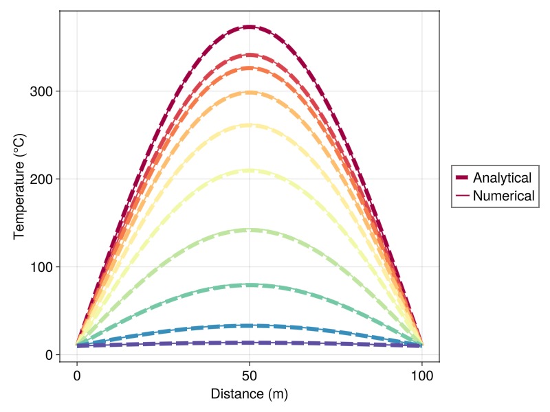

Piecewise constant initial conditions

We now consider a more challenging initial condition where the initial temperature profile is piecewise constant, with four different constant values.

T_0 = x ->
    to_kelvin(100.0) .* (x < 25) +
    to_kelvin(20.0) .* (25 <= x < 50) +
    to_kelvin(50.0) .* (50 <= x < 75) +
    to_kelvin(75.0) .* (75 <= x);

We can still compute the analytical solution using the formula above, but the sum will now be an infinite series. The function analytical_1d handles this pragmatically by truncating the series when the contribution of the next term is less than a 1e-6.

case, sol, x, t = analytical_1d(
    L=L, temperature_boundary=T_b, initial_condition=T_0,
    num_cells=500, num_steps=500);

results = simulate_reservoir(case, info_level=0)
plot_temperature_1d(case, results, sol, x, t, 10)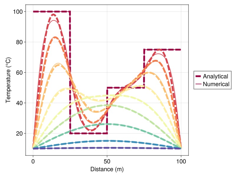

Numerical convergence analysis

We perform a comprehensive convergence study by systematically refining the spatial and temporal discretization. The default two-point flux approximation (TPFA) scheme used in JutulDarcy reduces to a central finite difference scheme for the heat equation, which is second-order accurate in space, whereas the implicit Backward Euler time integration is first-order accurate in time.

We use the same initial conditions as in the first example above

T_0 = x -> to_kelvin(90.0) .* sin(π * x / L) .+ T_b;
setup_case = (nx, nt) -> analytical_1d(
    L=L, temperature_boundary=T_b, initial_condition=T_0,
    num_cells=nx, num_steps=nt);

function convergence_1d(setup_fn, type=:space; Nx=2 .^ (range(3, 6)), Nt=2 .^ (range(3, 6)))
    if type == :space
        Nt = 10000
    elseif type == :time
        Nx = 10000
    else
        @assert type == :spacetime
        "Input type must be either :space, :time, or :spacetime"
    end
    Δx, Δt, err = [], [], []
    for nx in Nx
        dx = L / nx
        push!(Δx, dx)
        for nt in Nt
            out = setup_fn(nx, nt)
            case, sol, x, t = out
            dt = t[2] - t[1]
            push!(Δt, dt)

            sim, cfg = setup_reservoir_simulator(case;
                relaxation=true,
                tol_cnv=1e-8,
                info_level=0,
                max_timestep=Inf,
                timesteps=:none
            )
            cfg[:tolerances][:Reservoir][:default] = 1e-8

            results = simulate_reservoir(case, simulator=sim, config=cfg)
            ϵ = 0.0
            for k = 1:nt
                T_n = results.states[k][:Temperature]
                T_a = sol(x, t[k])
                ϵ += dt .* norm(dx .* (T_n .- T_a), 2)
            end

            push!(err, ϵ)
        end
    end
    err ./= err[1]
    return Δx, Δt, err

end

convergence_1d (generic function with 2 methods)

Spatial convergence analysis

We examine spatial convergence by systematically increasing the number of grid cells while using a very fine temporal discretization (10,000 timesteps) to eliminate temporal error contributions. The L2 norm of the error is computed over the entire space-time domain. We expect to observe second-order convergence as predicted by finite difference theory.

Δx, _, err_space = convergence_1d(setup_case, :space)

Δx ./= Δx[1]
opt = Δx .^ 2
fig = Figure(size=(800, 600), fontsize=20)
ax = Axis(fig[1, 1]; xlabel="Δx/Δx₀", ylabel="Error", xscale=log2, yscale=log2)
lines!(ax, Δx, opt, linewidth=4, color=:black, linestyle=:dash, label="2nd order")
scatter!(ax, Δx, err_space, marker=:rect, markersize=20, color=:black)
lines!(ax, Δx, err_space, linewidth=2, color=:black, label="Numerical")
Legend(fig[1, 2], ax)
fig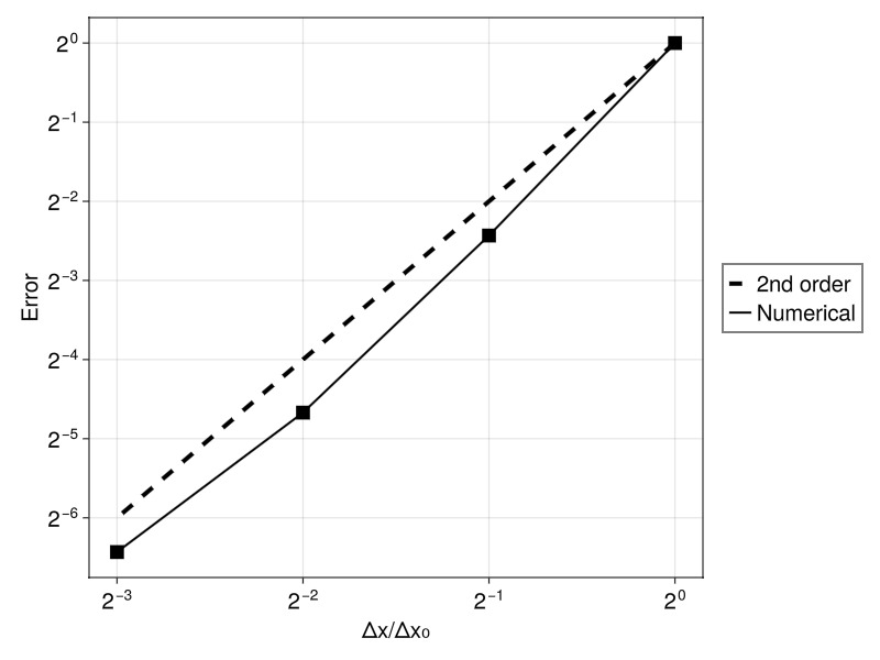

Temporal convergence analysis

We now study temporal convergence by using a very fine spatial discretization (10,000 cells) to eliminate spatial error contributions while systematically reducing the timestep size. We expect to observe first-order convergence characteristic of the implicit Backward Euler time integration scheme.

_, Δt, err_time = convergence_1d(setup_case, :time)

Δt ./= Δt[1]
opt = copy(Δt)
fig = Figure(size=(800, 600), fontsize=20)
ax = Axis(fig[1, 1]; xlabel="Δt/Δt₀", ylabel="Error", xscale=log2, yscale=log2)
lines!(ax, Δt, opt, linewidth=4, color=:black, linestyle=:dash, label="1st order")
scatter!(ax, Δt, err_time, marker=:rect, markersize=20, color=:black, label="Numerical")
lines!(ax, Δt, err_time, linewidth=2, color=:black)
Legend(fig[1, 2], ax)
fig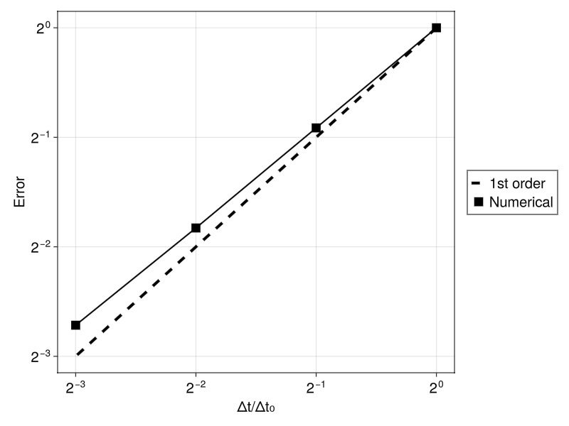

Example on GitHub

If you would like to run this example yourself, it can be downloaded from the Fimbul.jl GitHub repository as a script.

This example took 96.932164758 seconds to complete.

---

This page was generated using Literate.jl.