Borehole Thermal Energy Storage (BTES)
This example demonstrates how to set up and simulate seasonal Borehole Thermal Energy Storage (BTES) using Fimbul. The BTES system consists of multiple boreholes coupled in series and parallel.
using Jutul, JutulDarcy
using Fimbul
using HYPRE
using GLMakie
Set up simulation case
We create a BTES system with 48 wells that extend to 100 m depth. The system operates on a seasonal cycle: wells are charged during summer months (April to September) with hot water at 90°C, and discharged during winter months (October to March) with cold water at 10°C. This seasonal operation is simulated over a 4-year period to study the thermal energy storage performance.
case, sections = btes(num_wells = 48, depths = [0.0, 0.5, 100, 125],
    charge_months = ["April", "May", "June", "July", "August", "September"],
    discharge_months = ["October", "November", "December", "January", "February", "March"],
    num_years = 4,
);
Info : Clearing all models and views...
Info : Done clearing all models and views
Info : Meshing 1D...
Info : [ 0%] Meshing curve 1 (Line)
Info : [ 10%] Meshing curve 2 (Line)
Info : [ 10%] Meshing curve 3 (Line)
Info : [ 10%] Meshing curve 4 (Line)
Info : [ 10%] Meshing curve 5 (Line)
Info : [ 10%] Meshing curve 6 (Line)
Info : [ 10%] Meshing curve 7 (Line)
Info : [ 10%] Meshing curve 8 (Line)
Info : [ 20%] Meshing curve 9 (Line)
Info : [ 20%] Meshing curve 10 (Line)
Info : [ 20%] Meshing curve 11 (Line)
Info : [ 20%] Meshing curve 12 (Line)
Info : [ 20%] Meshing curve 13 (Line)
Info : [ 20%] Meshing curve 14 (Line)
Info : [ 20%] Meshing curve 15 (Line)
Info : [ 30%] Meshing curve 16 (Line)
Info : [ 30%] Meshing curve 17 (Line)
Info : [ 30%] Meshing curve 18 (Line)
Info : [ 30%] Meshing curve 19 (Line)
Info : [ 30%] Meshing curve 20 (Line)
Info : [ 30%] Meshing curve 21 (Line)
Info : [ 30%] Meshing curve 22 (Line)
Info : [ 30%] Meshing curve 23 (Line)
Info : [ 40%] Meshing curve 24 (Line)
Info : [ 40%] Meshing curve 25 (Line)
Info : [ 40%] Meshing curve 27 (Extruded)
Info : [ 40%] Meshing curve 28 (Extruded)
Info : [ 40%] Meshing curve 29 (Extruded)
Info : [ 40%] Meshing curve 30 (Extruded)
Info : [ 40%] Meshing curve 31 (Extruded)
Info : [ 50%] Meshing curve 32 (Extruded)
Info : [ 50%] Meshing curve 33 (Extruded)
Info : [ 50%] Meshing curve 34 (Extruded)
Info : [ 50%] Meshing curve 35 (Extruded)
Info : [ 50%] Meshing curve 36 (Extruded)
Info : [ 50%] Meshing curve 37 (Extruded)
Info : [ 50%] Meshing curve 38 (Extruded)
Info : [ 50%] Meshing curve 39 (Extruded)
Info : [ 60%] Meshing curve 40 (Extruded)
Info : [ 60%] Meshing curve 41 (Extruded)
Info : [ 60%] Meshing curve 42 (Extruded)
Info : [ 60%] Meshing curve 43 (Extruded)
Info : [ 60%] Meshing curve 44 (Extruded)
Info : [ 60%] Meshing curve 45 (Extruded)
Info : [ 60%] Meshing curve 46 (Extruded)
Info : [ 70%] Meshing curve 47 (Extruded)
Info : [ 70%] Meshing curve 48 (Extruded)
Info : [ 70%] Meshing curve 49 (Extruded)
Info : [ 70%] Meshing curve 50 (Extruded)
Info : [ 70%] Meshing curve 51 (Extruded)
Info : [ 70%] Meshing curve 53 (Extruded)
Info : [ 70%] Meshing curve 54 (Extruded)
Info : [ 70%] Meshing curve 58 (Extruded)
Info : [ 80%] Meshing curve 62 (Extruded)
Info : [ 80%] Meshing curve 66 (Extruded)
Info : [ 80%] Meshing curve 70 (Extruded)
Info : [ 80%] Meshing curve 74 (Extruded)
Info : [ 80%] Meshing curve 78 (Extruded)
Info : [ 80%] Meshing curve 82 (Extruded)
Info : [ 80%] Meshing curve 86 (Extruded)
Info : [ 90%] Meshing curve 90 (Extruded)
Info : [ 90%] Meshing curve 94 (Extruded)
Info : [ 90%] Meshing curve 98 (Extruded)
Info : [ 90%] Meshing curve 102 (Extruded)
Info : [ 90%] Meshing curve 106 (Extruded)
Info : [ 90%] Meshing curve 110 (Extruded)
Info : [ 90%] Meshing curve 114 (Extruded)
Info : [ 90%] Meshing curve 118 (Extruded)
Info : [100%] Meshing curve 122 (Extruded)
Info : [100%] Meshing curve 126 (Extruded)
Info : [100%] Meshing curve 130 (Extruded)
Info : [100%] Meshing curve 134 (Extruded)
Info : [100%] Meshing curve 138 (Extruded)
Info : [100%] Meshing curve 142 (Extruded)
Info : [100%] Meshing curve 146 (Extruded)
Info : Done meshing 1D (Wall 0.00173574s, CPU 0.001737s)
Info : Meshing 2D...
Info : [ 0%] Meshing surface 1 (Plane, Frontal-Delaunay)
Warning : Cannot apply Blossom: odd number of triangles (2251) in surface 1
Info : [ 0%] Blossom recombination completed (Wall 0.0243523s, CPU 0.024352s): 982 quads, 279 triangles, 0 invalid quads, 2 quads with Q < 0.1, avg Q = 0.760482, min Q = 0.0452156
Info : [ 10%] Meshing surface 55 (Extruded)
Info : [ 10%] Meshing surface 59 (Extruded)
Info : [ 20%] Meshing surface 63 (Extruded)
Info : [ 20%] Meshing surface 67 (Extruded)
Info : [ 20%] Meshing surface 71 (Extruded)
Info : [ 30%] Meshing surface 75 (Extruded)
Info : [ 30%] Meshing surface 79 (Extruded)
Info : [ 30%] Meshing surface 83 (Extruded)
Info : [ 40%] Meshing surface 87 (Extruded)
Info : [ 40%] Meshing surface 91 (Extruded)
Info : [ 50%] Meshing surface 95 (Extruded)
Info : [ 50%] Meshing surface 99 (Extruded)
Info : [ 50%] Meshing surface 103 (Extruded)
Info : [ 60%] Meshing surface 107 (Extruded)
Info : [ 60%] Meshing surface 111 (Extruded)
Info : [ 60%] Meshing surface 115 (Extruded)
Info : [ 70%] Meshing surface 119 (Extruded)
Info : [ 70%] Meshing surface 123 (Extruded)
Info : [ 80%] Meshing surface 127 (Extruded)
Info : [ 80%] Meshing surface 131 (Extruded)
Info : [ 80%] Meshing surface 135 (Extruded)
Info : [ 90%] Meshing surface 139 (Extruded)
Info : [ 90%] Meshing surface 143 (Extruded)
Info : [ 90%] Meshing surface 147 (Extruded)
Info : [100%] Meshing surface 151 (Extruded)
Info : [100%] Meshing surface 152 (Extruded)
Info : Done meshing 2D (Wall 0.0513926s, CPU 0.051391s)
Info : Meshing 3D...
Info : Meshing volume 1 (Extruded)
Info : Done meshing 3D (Wall 0.15447s, CPU 0.154449s)
Info : Optimizing mesh...
Info : Done optimizing mesh (Wall 0.00064782s, CPU 0.000648s)
Info : 27240 nodes 32823 elements
Warning : ------------------------------
Warning : Mesh generation error summary
Warning : 1 warning
Warning : 0 errors
Warning : Check the full log for details
Warning : ------------------------------
Info : Removing duplicate mesh nodes...
Info : Found 0 duplicate nodes
Info : No duplicate nodes found
Adding well B1 (1/48)
Adding well B2 (2/48)
Adding well B3 (3/48)
Adding well B4 (4/48)
Adding well B5 (5/48)
Adding well B6 (6/48)
Adding well B7 (7/48)
Adding well B8 (8/48)
Adding well B9 (9/48)
Adding well B10 (10/48)
Adding well B11 (11/48)
Adding well B12 (12/48)
Adding well B13 (13/48)
Adding well B14 (14/48)
Adding well B15 (15/48)
Adding well B16 (16/48)
Adding well B17 (17/48)
Adding well B18 (18/48)
Adding well B19 (19/48)
Adding well B20 (20/48)
Adding well B21 (21/48)
Adding well B22 (22/48)
Adding well B23 (23/48)
Adding well B24 (24/48)
Adding well B25 (25/48)
Adding well B26 (26/48)
Adding well B27 (27/48)
Adding well B28 (28/48)
Adding well B29 (29/48)
Adding well B30 (30/48)
Adding well B31 (31/48)
Adding well B32 (32/48)
Adding well B33 (33/48)
Adding well B34 (34/48)
Adding well B35 (35/48)
Adding well B36 (36/48)
Adding well B37 (37/48)
Adding well B38 (38/48)
Adding well B39 (39/48)
Adding well B40 (40/48)
Adding well B41 (41/48)
Adding well B42 (42/48)
Adding well B43 (43/48)
Adding well B44 (44/48)
Adding well B45 (45/48)
Adding well B46 (46/48)
Adding well B47 (47/48)
Adding well B48 (48/48)Visualize BTES system layout
The 48 BTES wells are arranged in a pattern that ensures approximately equal spacing between wells. The wells are organized into 6 sections of 8 wells each. During charging, water is injected at 0.5 l/s into the innermost well of each section and flows sequentially through all wells in series to the outermost well. During discharging, the flow direction reverses, with water flowing from the outermost well back to the innermost well.
msh = physical_representation(reservoir_model(case.model).data_domain)
fig = Figure(size = (800, 800))
ax = Axis3(fig[1, 1]; zreversed = true, aspect = :data,
azimuth = 0, elevation = π/2)
Jutul.plot_mesh_edges!(ax, msh, alpha = 0.2)
colors = Makie.wong_colors()
lns, labels = [], String[]
for (sno, (section, wells)) in enumerate(sections)
    for (wno, wname) in enumerate(wells)
        well = case.model.models[wname].domain.representation
        l = plot_well!(ax, msh, well; color = colors[sno], fontsize = 0)
        if wno == 1
            push!(lns, l)
            push!(labels, "Section $sno")
        end
    end
end
Legend(fig[1, 2], lns, labels);
fig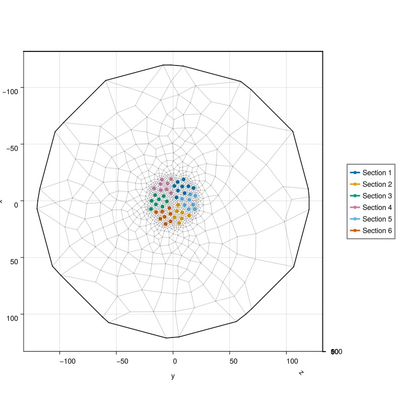
Set up reservoir simulator
We configure the simulator with specific tolerances and timestep controls to handle the challenging thermal transients in the BTES system.
simulator, config = setup_reservoir_simulator(case;
    tol_cnv = 1e-2,
    tol_mb = 1e-6,
    timesteps = :auto,
    initial_dt = 5.0,
    relaxation = true);
The transition from charging to discharging creates a thermal shock that is numerically challenging for the nonlinear solver. We use a specialized timestep selector that reduces the timestep to 5 seconds during control changes to maintain numerical stability and convergence.
sel = JutulDarcy.ControlChangeTimestepSelector(
    case.model, 0.0, convert_to_si(5.0, :second))
push!(config[:timestep_selectors], sel)
config[:timestep_max_decrease] = 1e-6
for ws in well_symbols(case.model)
    config[:tolerances][ws][:default] = 1e-2
end
Simulate the BTES system
Run the full 4-year simulation with the configured solver settings.
Note that this simulation can take a few minutes to run. Setting info_level = 0 will show a progress bar while the simulation runs.`
results = simulate_reservoir(case;
simulator=simulator, config=config, info_level=-1);
╭────────────────┬──────────┬───────────────┬────────────╮
│ Iteration type │ Avg/step │ Avg/ministep │ Total │
│ │ 96 steps │ 978 ministeps │ (wasted) │
├────────────────┼──────────┼───────────────┼────────────┤
│ Newton │ 64.2708 │ 6.30879 │ 6170 (10) │
│ Linearization │ 74.4062 │ 7.30368 │ 7143 (10) │
│ Linear solver │ 112.969 │ 11.089 │ 10845 (5) │
│ Precond apply │ 225.938 │ 22.1779 │ 21690 (10) │
╰────────────────┴──────────┴───────────────┴────────────╯
╭───────────────┬──────────┬────────────┬──────────╮
│ Timing type │ Each │ Relative │ Total │
│ │ ms │ Percentage │ s │
├───────────────┼──────────┼────────────┼──────────┤
│ Properties │ 4.4626 │ 3.58 % │ 27.5341 │
│ Equations │ 42.0272 │ 39.04 % │ 300.2003 │
│ Assembly │ 9.6705 │ 8.98 % │ 69.0762 │
│ Linear solve │ 3.4078 │ 2.73 % │ 21.0259 │
│ Linear setup │ 40.4726 │ 32.48 % │ 249.7161 │
│ Precond apply │ 2.9142 │ 8.22 % │ 63.2096 │
│ Update │ 1.6404 │ 1.32 % │ 10.1212 │
│ Convergence │ 2.2748 │ 2.11 % │ 16.2488 │
│ Input/Output │ 0.3055 │ 0.04 % │ 0.2988 │
│ Other │ 1.8652 │ 1.50 % │ 11.5085 │
├───────────────┼──────────┼────────────┼──────────┤
│ Total │ 124.6255 │ 100.00 % │ 768.9394 │
╰───────────────┴──────────┴────────────┴──────────╯Interactive visualization of results
We first plot the final temperature distribution in the reservoir and well performance over time. The reservoir plot shows the thermal plumes developed around each well section, while the well results show the temperature and flow rate evolution throughout the simulation.
plot_reservoir(case.model, results.states;
well_fontsize = 0, key = :Temperature, step = length(case.dt),
colormap = :seaborn_icefire_gradient)

plot_well_results(results.wells, field = :temperature)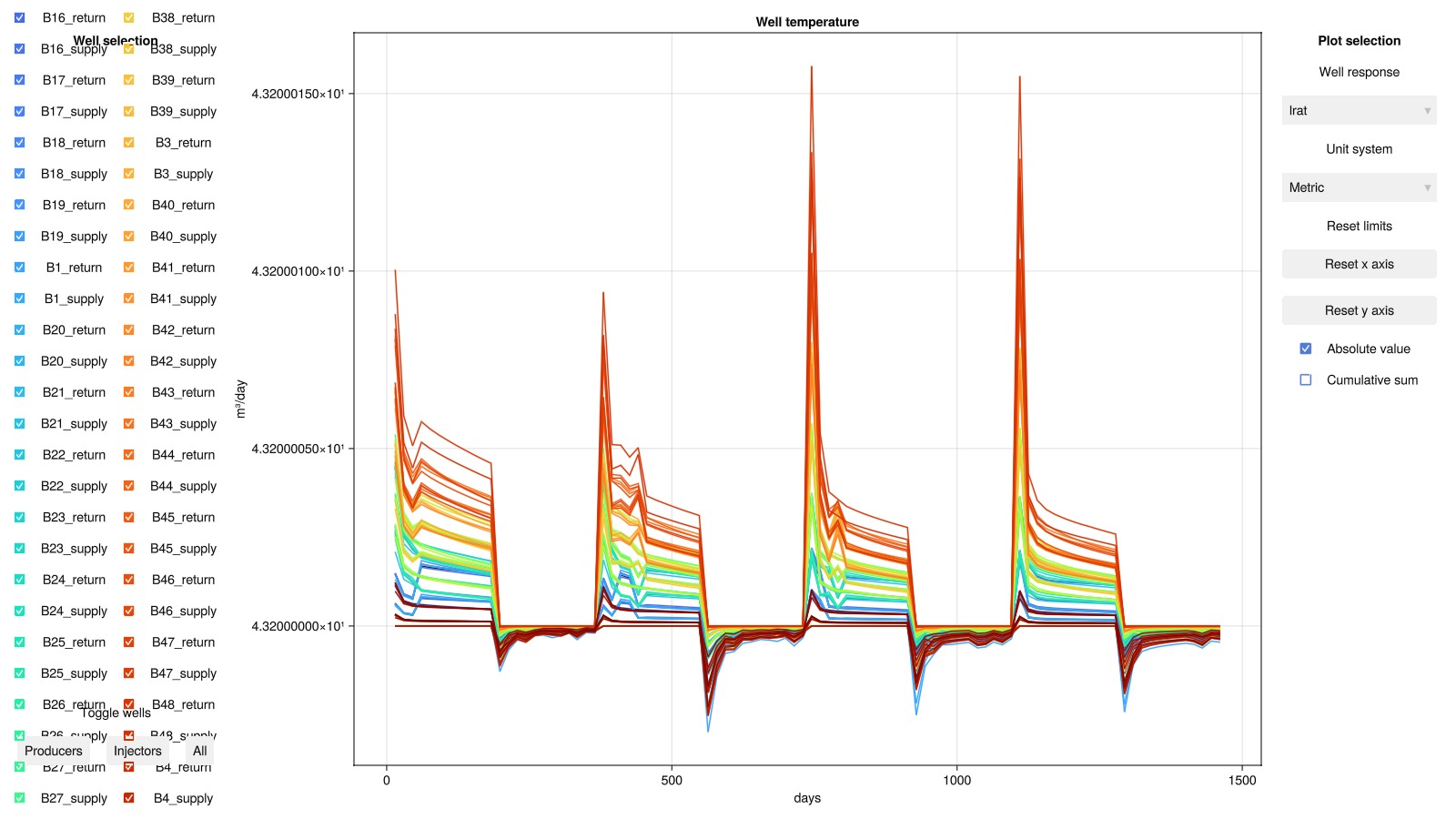
Temperature evolution in the reservoir
Next, we visualize how thermal energy storage develops in the subsurface over time. We examine the temperature distribution after each of the four charging cycles to see how the thermal plume grows. For better visualization, we only display cells below 50 m depth with temperatures above 15°C (warmer than the natural ground temperature).
dstep = Int64.(length(case.dt)/(4*2))
steps = dstep:2*dstep:length(case.dt)
fig = Figure(size = (1000, 750))
geo = tpfv_geometry(msh)
bottom = geo.cell_centroids[3,:] .>= 50.0
T_min, T_max = Inf, -Inf
for (sno, step) in enumerate(steps)
    ax_sno = Axis3(fig[(sno-1)÷2+1, (sno-1)%2+1];
    limits = (-50, 50, -50, 50, 40, 125),
    title = "Charge $sno", zreversed = true, aspect = :data)
    T = convert_from_si.(results.states[step][:Temperature], :Celsius)
    cells = bottom .& (T .>= 15.0)
    global T_min = min(T_min, minimum(T[cells]))
    global T_max = max(T_max, maximum(T[cells]))
    plot_cell_data!(ax_sno, msh, T; cells = cells, colormap = :seaborn_icefire_gradient)
    hidedecorations!(ax_sno)
end
Colorbar(fig[1:2, 3];
colormap = :seaborn_icefire_gradient, colorrange = (T_min, T_max),
label = "T ≥ 15.0 °C", vertical = true)
fig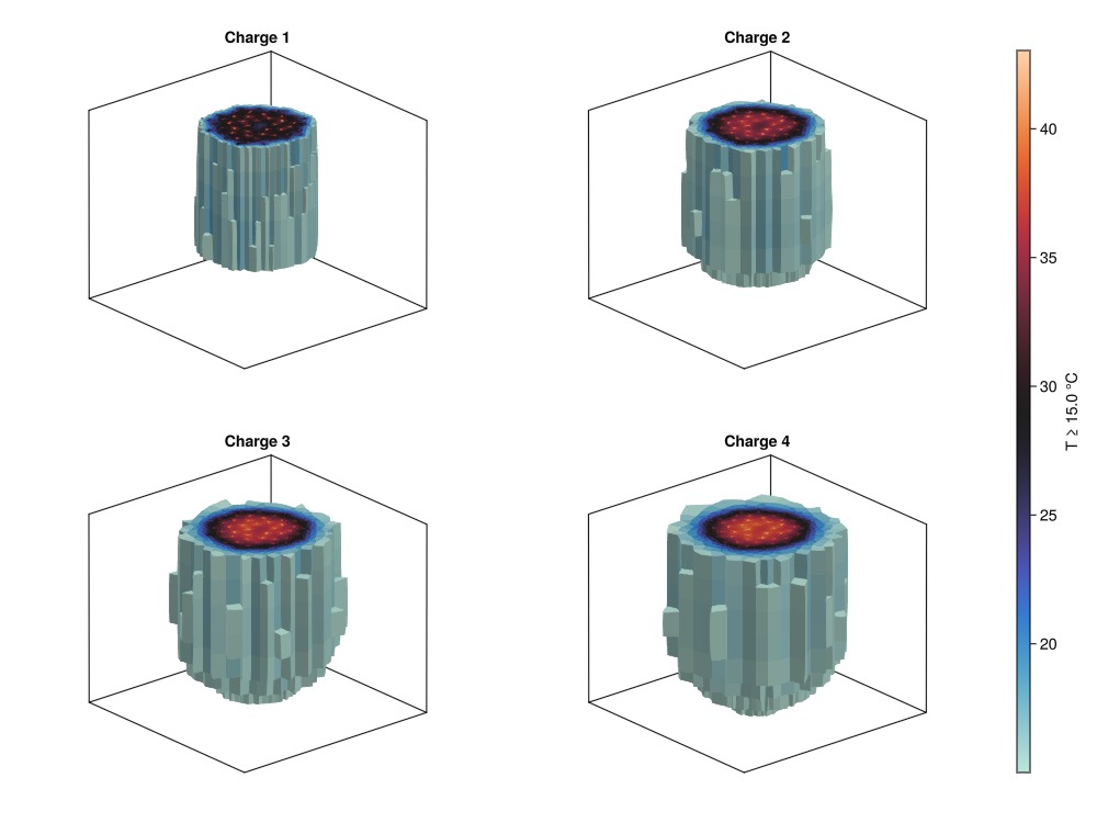
Temperature evolution within the boreholes
Understanding the temperature profiles within individual boreholes is crucial for BTES system design. We analyze how temperature varies with depth along the wellbore during both charging and discharging phases. This information can help determine optimal well depth, number of wells needed, and the most effective series/parallel coupling configuration for a given thermal storage capacity requirement.
To this end, we define a utility function to plot temperature evolution in a BTES section. This function visualizes temperature as a function of well depth for all wells in a given section at specified timesteps, helping to understand thermal propagation through the wellbore network.
function plot_btes_temperature(ax, section, timesteps)
    colors = cgrad(:ice, length(timesteps), categorical = true)
    msh = physical_representation(reservoir_model(case.model).data_domain)
    geo = tpfv_geometry(msh)
    time = convert_from_si.(cumsum(case.dt), :day)
    out = []
    for (sno, step) in enumerate(timesteps)
        label = String("$(time[step]) days")
        for (wno, well) in enumerate(sections[Symbol("S$section")])
            lbl = wno == 1 ? label : nothing
            T = results.result.states[step][well][:Temperature]
            T = convert_from_si.(T, :Celsius)
            wm = case.model.models[well]
            num_nodes = length(wm.domain.representation.perforations.reservoir)
            plot_mswell_values!(ax, case.model, well, T;
            nodes = 1:num_nodes, geo = geo, color = colors[sno], linewidth = 6, label = lbl)
        end
    end
end

fig = Figure(size = (1000, 750))
section = 11Temperature evolution during the first charging cycle
We first visualize how thermal energy propagates through the wellbore network as hot water flows from the innermost to the outermost well in the section.
well = sections[Symbol("S$section")][1]
T_ch = convert_to_si(90.0, :Celsius)
is_charge = [f[:Facility].control[well].temperature == T_ch for f in case.forces]
stop = findfirst(diff(is_charge) .< 0)
ax = Axis(fig[1, 1]; title = "Temperature evolution, section $section (charging)",
xlabel = "T [°C]", ylabel = "Depth [m]", yreversed = true)
plot_btes_temperature(ax, section, 1:stop)
Legend(fig[1,2], ax; fontsize = 20)Makie.Legend()Temperature evolution during the first discharging cycle
Next, we show how stored thermal energy is extracted as flow direction reverses, with water flowing from the outermost to the innermost well.
well = sections[Symbol("S$section")][end-1]
T_dch = convert_to_si(10.0, :Celsius)
is_discharge = [f[:Facility].control[well].temperature == T_dch for f in case.forces]
start = findfirst(diff(is_discharge) .> 0)+1
stop = findfirst(diff(is_discharge) .< 0)
ax = Axis(fig[2, 1]; title = "Temperature evolution, section $section (discharging)",
xlabel = "T [°C]", ylabel = "Depth [m]", yreversed = true)
plot_btes_temperature(ax, section, start:stop)
Legend(fig[2,2], ax; fontsize = 20)

fig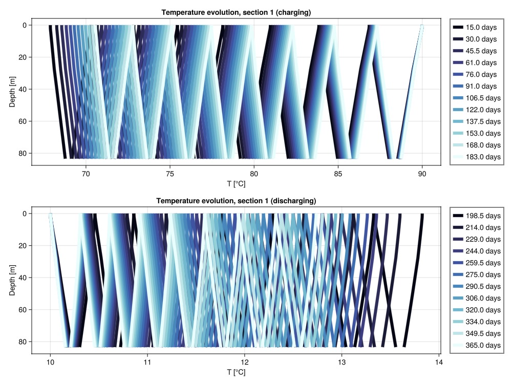
Example on GitHub
If you would like to run this example yourself, it can be downloaded from the Fimbul.jl GitHub repository as a script.
This example took 814.056646302 seconds to complete.This page was generated using Literate.jl.