Geothermal energy production from a well doublet

This example demonstrates how to simulate and visualize the production of geothermal energy from a doublet well system. The setup consists of a producer well that extracts hot water from the reservoir, and an injector well that reinjects produced water at a lower temperature.

Add required modules to namespace

using Jutul, JutulDarcy, Fimbul
using HYPRE
using GLMakie

Set up case

The injector and producer wells are placed 100 m apart at the top, and run parallel down to 800 m depth before they diverge to a distance of 1000 m at 2500 m depth.

case, plot_args = geothermal_doublet();

Info    : Clearing all models and views...
Info    : Done clearing all models and views
Info    : Meshing 1D...
Info    : [  0%] Meshing curve 1 (Line)
Info    : [ 10%] Meshing curve 2 (Line)
Info    : [ 10%] Meshing curve 3 (Line)
Info    : [ 10%] Meshing curve 4 (Line)
Info    : [ 10%] Meshing curve 5 (Line)
Info    : [ 10%] Meshing curve 6 (Line)
Info    : [ 20%] Meshing curve 7 (Line)
Info    : [ 20%] Meshing curve 8 (Line)
Info    : [ 20%] Meshing curve 9 (Line)
Info    : [ 20%] Meshing curve 10 (Line)
Info    : [ 20%] Meshing curve 11 (Line)
Info    : [ 30%] Meshing curve 12 (Line)
Info    : [ 30%] Meshing curve 13 (Line)
Info    : [ 30%] Meshing curve 14 (Line)
Info    : [ 30%] Meshing curve 15 (Line)
Info    : [ 30%] Meshing curve 16 (Line)
Info    : [ 40%] Meshing curve 17 (Line)
Info    : [ 40%] Meshing curve 18 (Line)
Info    : [ 40%] Meshing curve 19 (Line)
Info    : [ 40%] Meshing curve 21 (Extruded)
Info    : [ 40%] Meshing curve 22 (Extruded)
Info    : [ 40%] Meshing curve 23 (Extruded)
Info    : [ 50%] Meshing curve 24 (Extruded)
Info    : [ 50%] Meshing curve 25 (Extruded)
Info    : [ 50%] Meshing curve 26 (Extruded)
Info    : [ 50%] Meshing curve 27 (Extruded)
Info    : [ 50%] Meshing curve 28 (Extruded)
Info    : [ 60%] Meshing curve 29 (Extruded)
Info    : [ 60%] Meshing curve 30 (Extruded)
Info    : [ 60%] Meshing curve 31 (Extruded)
Info    : [ 60%] Meshing curve 32 (Extruded)
Info    : [ 60%] Meshing curve 33 (Extruded)
Info    : [ 70%] Meshing curve 34 (Extruded)
Info    : [ 70%] Meshing curve 35 (Extruded)
Info    : [ 70%] Meshing curve 36 (Extruded)
Info    : [ 70%] Meshing curve 37 (Extruded)
Info    : [ 70%] Meshing curve 39 (Extruded)
Info    : [ 70%] Meshing curve 40 (Extruded)
Info    : [ 80%] Meshing curve 44 (Extruded)
Info    : [ 80%] Meshing curve 48 (Extruded)
Info    : [ 80%] Meshing curve 52 (Extruded)
Info    : [ 80%] Meshing curve 56 (Extruded)
Info    : [ 80%] Meshing curve 60 (Extruded)
Info    : [ 90%] Meshing curve 64 (Extruded)
Info    : [ 90%] Meshing curve 68 (Extruded)
Info    : [ 90%] Meshing curve 72 (Extruded)
Info    : [ 90%] Meshing curve 76 (Extruded)
Info    : [ 90%] Meshing curve 80 (Extruded)
Info    : [100%] Meshing curve 84 (Extruded)
Info    : [100%] Meshing curve 88 (Extruded)
Info    : [100%] Meshing curve 92 (Extruded)
Info    : [100%] Meshing curve 96 (Extruded)
Info    : [100%] Meshing curve 100 (Extruded)
Info    : Done meshing 1D (Wall 0.00529429s, CPU 0.005296s)
Info    : Meshing 2D...
Info    : [  0%] Meshing surface 1 (Plane, Frontal-Delaunay)
Warning : Cannot apply Blossom: odd number of triangles (2575) in surface 1
Info    : [  0%] Blossom recombination completed (Wall 0.0249499s, CPU 0.02495s): 1122 quads, 321 triangles, 0 invalid quads, 0 quads with Q < 0.1, avg Q = 0.764788, min Q = 0.308496
Info    : [ 10%] Meshing surface 41 (Extruded)
Info    : [ 20%] Meshing surface 45 (Extruded)
Info    : [ 20%] Meshing surface 49 (Extruded)
Info    : [ 30%] Meshing surface 53 (Extruded)
Info    : [ 30%] Meshing surface 57 (Extruded)
Info    : [ 40%] Meshing surface 61 (Extruded)
Info    : [ 40%] Meshing surface 65 (Extruded)
Info    : [ 50%] Meshing surface 69 (Extruded)
Info    : [ 50%] Meshing surface 73 (Extruded)
Info    : [ 60%] Meshing surface 77 (Extruded)
Info    : [ 60%] Meshing surface 81 (Extruded)
Info    : [ 70%] Meshing surface 85 (Extruded)
Info    : [ 70%] Meshing surface 89 (Extruded)
Info    : [ 80%] Meshing surface 93 (Extruded)
Info    : [ 80%] Meshing surface 97 (Extruded)
Info    : [ 90%] Meshing surface 101 (Extruded)
Info    : [ 90%] Meshing surface 105 (Extruded)
Info    : [100%] Meshing surface 106 (Extruded)
Info    : Done meshing 2D (Wall 0.0600044s, CPU 0.060003s)
Info    : Meshing 3D...
Info    : Meshing volume 1 (Extruded)
Info    : Done meshing 3D (Wall 0.37294s, CPU 0.372902s)
Info    : Optimizing mesh...
Info    : Done optimizing mesh (Wall 0.00232945s, CPU 0.002328s)
Info    : 74100 nodes 86626 elements
Warning : ------------------------------
Warning : Mesh generation error summary
Warning :     1 warning
Warning :     0 errors
Warning : Check the full log for details
Warning : ------------------------------
Info    : Removing duplicate mesh nodes...
Info    : Found 0 duplicate nodes
Info    : No duplicate nodes found

Inspect model

We first plot the computational mesh and wells. The mesh is refined around the wells in the horizontal plane and vertically in and near the target aquifer.

msh = physical_representation(reservoir_model(case.model).data_domain)
fig = Figure(size = (1200, 800))
ax = Axis3(fig[1, 1], zreversed = true, aspect = plot_args.aspect)
Jutul.plot_mesh_edges!(ax, msh, alpha = 1.0)
wells = get_model_wells(case.model)
for (k, w) in wells
    plot_well!(ax, msh, w)
end
fig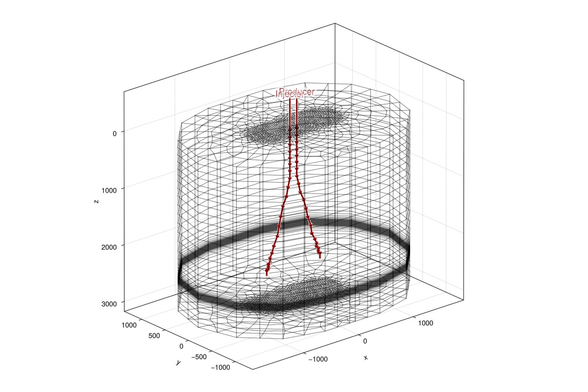

Plot reservoir properties

Next, we visualize the reservoir interactively.

plot_reservoir(case.model; plot_args...)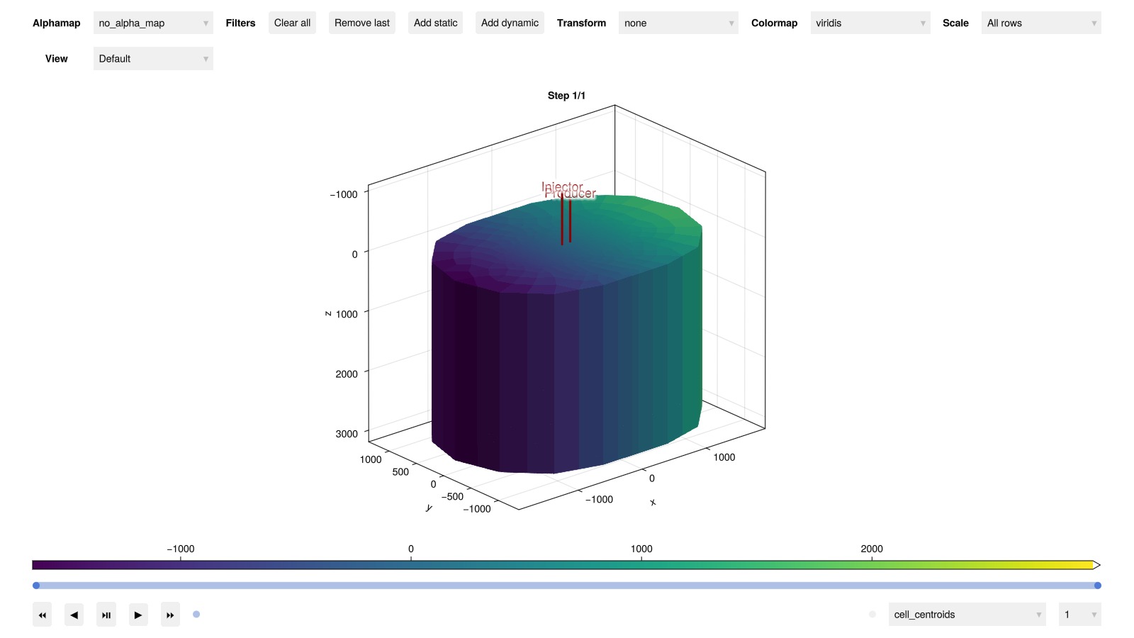

Simulate geothermal energy production

We simulate the geothermal doublet for 200 years. The producer is set to produce at a rate of 300 m^3/hour with a lower BHP limit of 1 bar, while the injector is set to reinject the produced water, lowered to a temperature of 20 °C.

Note: this simulation can take a few minutes to run. Setting info_level = 0 will show a progress bar while the simulation runs.

results = simulate_reservoir(case; info_level = -1)

ReservoirSimResult with 200 entries:

  wells (2 present):
    :Producer
    :Injector
    Results per well:
       :lrat => Vector{Float64} of size (200,)
       :wrat => Vector{Float64} of size (200,)
       :temperature => Vector{Float64} of size (200,)
       :control => Vector{Symbol} of size (200,)
       :Aqueous_mass_rate => Vector{Float64} of size (200,)
       :bhp => Vector{Float64} of size (200,)
       :wcut => Vector{Float64} of size (200,)
       :mass_rate => Vector{Float64} of size (200,)
       :rate => Vector{Float64} of size (200,)

  states (Vector with 200 entries, reservoir variables for each state)
    :Pressure => Vector{Float64} of size (80808,)
    :TotalMasses => Matrix{Float64} of size (1, 80808)
    :TotalThermalEnergy => Vector{Float64} of size (80808,)
    :FluidEnthalpy => Matrix{Float64} of size (1, 80808)
    :Temperature => Vector{Float64} of size (80808,)
    :PhaseMassDensities => Matrix{Float64} of size (1, 80808)
    :RockInternalEnergy => Vector{Float64} of size (80808,)
    :FluidInternalEnergy => Matrix{Float64} of size (1, 80808)
    :PhaseViscosities => Matrix{Float64} of size (1, 80808)

  time (report time for each state)
     Vector{Float64} of length 200

  result (extended states, reports)
     SimResult with 200 entries

  extra
     Dict{Any, Any} with keys :simulator, :config

  Completed at Jul. 07 2025 22:07 after 3 minutes, 15 seconds, 811.1 milliseconds.

Visualize results

We first plot the reservoir state interactively. You can notice how the cold front propagates from the injector well by filtering out high values.

plot_reservoir(case.model, results.states;
colormap = :seaborn_icefire_gradient, key = :Temperature, plot_args...)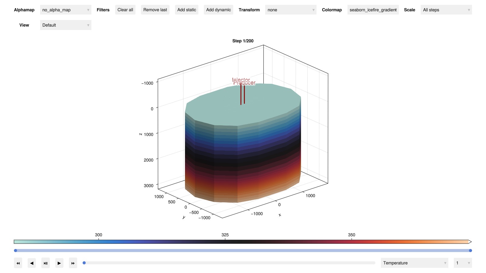

Plot well output

Next, we plot the well output to examine the production rates and temperatures.

plot_well_results(results.wells)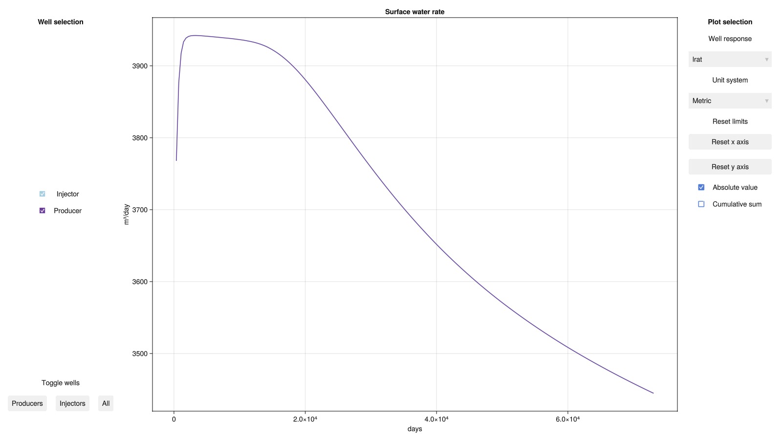

Well temperature evolution

For a more detailed analysis of the production temperature evolution, we plot the temperature inside the production well as a function of well depth for all 200 years of production. We also highlight the temperature at selected timesteps (7, 21, 65, and 200 years).

states = results.result.states
times = convert_from_si.(cumsum(case.dt), :year)
geo = tpfv_geometry(msh)

fig = Figure(size = (1200, 800))
ax = Axis(fig[1, 1], xlabel = "Temperature (°C)", ylabel = "Depth (m)", yreversed = true)
colors = cgrad(:seaborn_icefire_gradient, length(states), categorical = true)

Plot temperature profiles for all timesteps with transparency

for (n, state) in enumerate(states)
    T = convert_from_si.(state[:Producer][:Temperature], :Celsius)
    plot_mswell_values!(ax, case.model, :Producer, T;
    geo = geo, linewidth = 4, color = colors[n], alpha = 0.25)
end

Highlight selected timesteps with solid lines and labels

timesteps = [7, 21, 65, 200]
for n in timesteps
    T = convert_from_si.(states[n][:Producer][:Temperature], :Celsius)
    plot_mswell_values!(ax, case.model, :Producer, T;
    geo = geo, linewidth = 4, color = colors[n], label = "$(times[n]) years")
end
axislegend(ax; position = :lt, fontsize = 20)
fig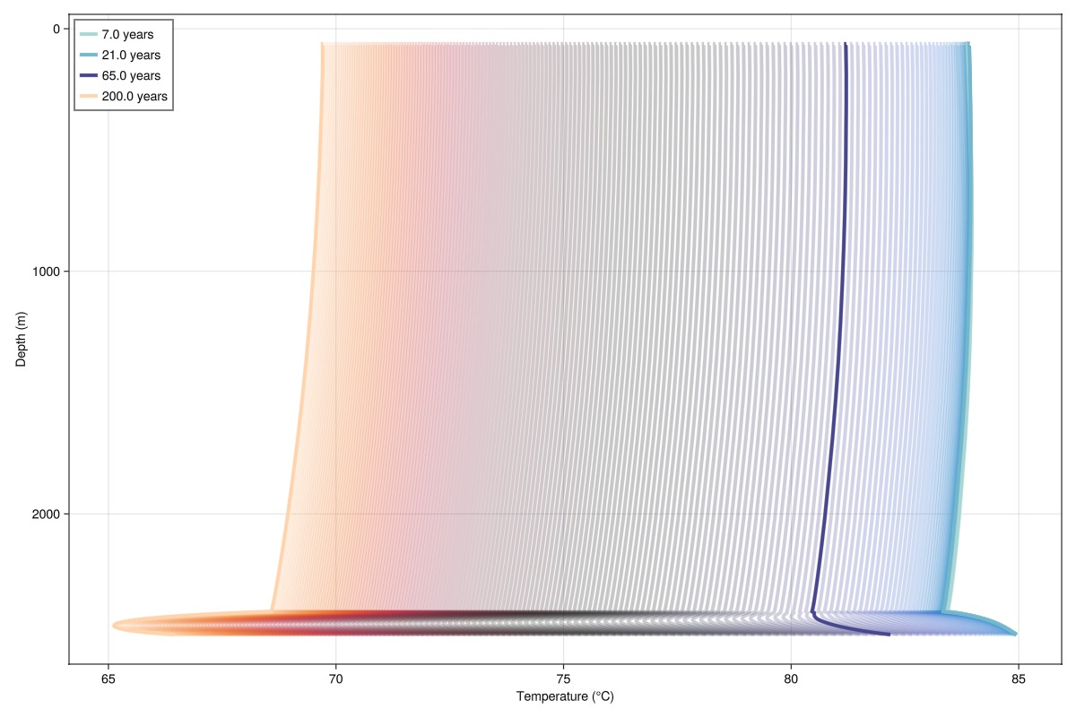

We can clearly see the footprint of the cold front in the aquifer (2400-2500 m depth) as it approaches the production well.

Reservoir state evolution

Another informative plot is the change in reservoir states over time. We compute the change in reservoir states from the initial state and plot the results interactively. The change in temperature is particularly interesting as it shows the evolution of the cold front in the aquifer

Δstates = []
for state in results.states
    Δstate = Dict{Symbol, Any}()
    for (k, v) in state
        v0 = case.state0[:Reservoir][k]
        Δstate[k] = v .- v0
    end
    push!(Δstates, Δstate)
end
plot_reservoir(case.model, Δstates;
colormap = :seaborn_icefire_gradient, key = :Temperature, plot_args...)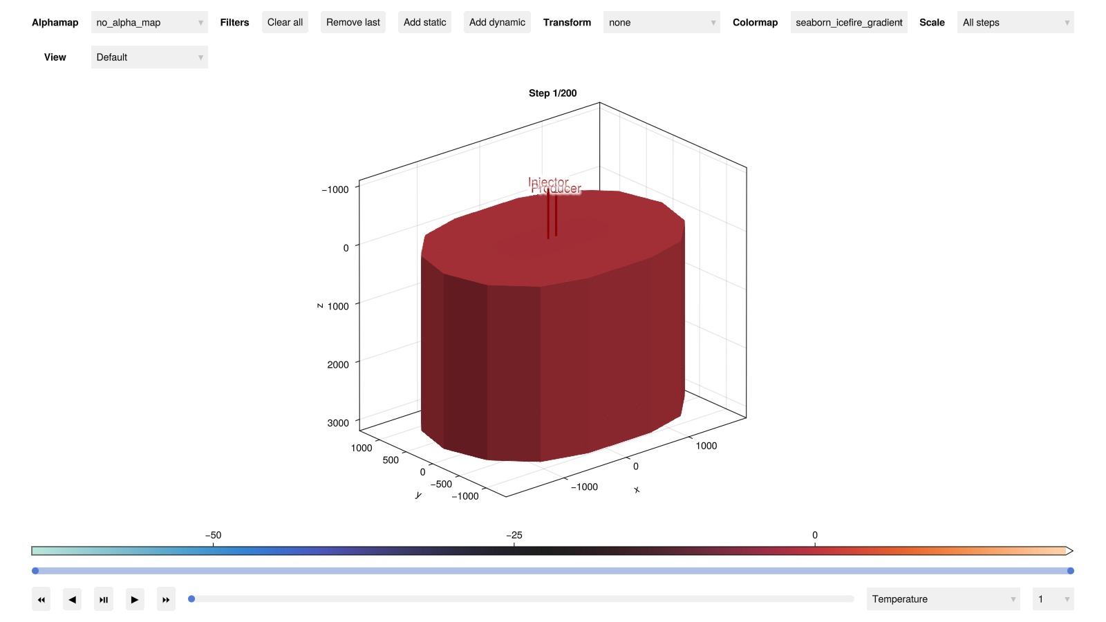

3D visualization of temperature changes

Finally, we plot the change in temperature at the same timesteps highlighted in the production well temperature above. We cut away parts of the model for better visualization. Define the temperature range and create a mask to cut away parts of the model

T_min = minimum(Δstates[end][:Temperature])
T_max = maximum(Δstates[1][:Temperature])
cells = geo.cell_centroids[1, :] .> -1000.0/2
cells = cells .&& geo.cell_centroids[2, :] .> 50.0
cells = cells .|| geo.cell_centroids[3, :] .> 2475.0

80808-element BitVector:
 0
 0
 0
 0
 0
 0
 0
 0
 0
 0
 ⋮
 1
 1
 1
 1
 1
 1
 1
 1
 1

Create subplots for each highlighted timestep

fig = Figure(size = (800, 800))
for (i, n) in enumerate(timesteps)
    ax = Axis3(fig[(i-1)÷2+1, (i-1)%2+1]; title = "$(times[n]) years",
    zreversed = true, elevation = pi/8, aspect = :data)

    ΔT = Δstates[n][:Temperature]

    plot_cell_data!(ax, msh, ΔT;
        cells = cells, colormap = :seaborn_icefire_gradient, colorrange = (T_min, T_max))
    plot_well!(ax, msh, wells[:Injector];
    color = :black, linewidth = 4, top_factor = 0.4, markersize = 0.0)
    plot_well!(ax, msh, wells[:Producer];
    color = :black, linewidth = 4, markersize = 0.0)
    hidedecorations!(ax)
end
Colorbar(fig[3, 1:2];
    colormap = :seaborn_icefire_gradient, colorrange = (T_min, T_max),
    label = "ΔT (°C)", vertical = false)
fig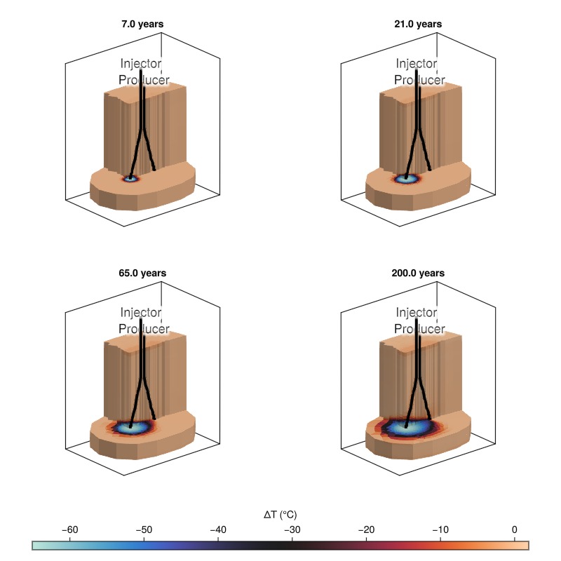

Example on GitHub

If you would like to run this example yourself, it can be downloaded from the Fimbul.jl GitHub repository as a script.

This example took 295.1396488 seconds to complete.

---

This page was generated using Literate.jl.