Borehole Thermal Energy Storage (BTES)
Storage BTESThis example demonstrates how to set up and simulate seasonal Borehole Thermal Energy Storage (BTES) using Fimbul. The BTES system consists of multiple boreholes coupled in series and parallel.
using Jutul, JutulDarcy
using Fimbul
using HYPRE
using GLMakie
Set up simulation case
We create a BTES system with 48 wells that extend to 100 m depth. The system operates on a seasonal cycle: wells are charged during summer months (April to September) with hot water at 90°C, and discharged during winter months (October to March) with cold water at 10°C. This seasonal operation is simulated over a 4-year period to study the thermal energy storage performance.
case = btes(num_wells = 48, depths = [0.0, 0.5, 100, 125],
    charge_period = ["April", "September"],
    discharge_period = ["October", "March"],
    num_years = 4,
);
Adding well B1 (1/48)
Adding well B2 (2/48)
Adding well B3 (3/48)
Adding well B4 (4/48)
Adding well B5 (5/48)
Adding well B6 (6/48)
Adding well B7 (7/48)
Adding well B8 (8/48)
Adding well B9 (9/48)
Adding well B10 (10/48)
Adding well B11 (11/48)
Adding well B12 (12/48)
Adding well B13 (13/48)
Adding well B14 (14/48)
Adding well B15 (15/48)
Adding well B16 (16/48)
Adding well B17 (17/48)
Adding well B18 (18/48)
Adding well B19 (19/48)
Adding well B20 (20/48)
Adding well B21 (21/48)
Adding well B22 (22/48)
Adding well B23 (23/48)
Adding well B24 (24/48)
Adding well B25 (25/48)
Adding well B26 (26/48)
Adding well B27 (27/48)
Adding well B28 (28/48)
Adding well B29 (29/48)
Adding well B30 (30/48)
Adding well B31 (31/48)
Adding well B32 (32/48)
Adding well B33 (33/48)
Adding well B34 (34/48)
Adding well B35 (35/48)
Adding well B36 (36/48)
Adding well B37 (37/48)
Adding well B38 (38/48)
Adding well B39 (39/48)
Adding well B40 (40/48)
Adding well B41 (41/48)
Adding well B42 (42/48)
Adding well B43 (43/48)
Adding well B44 (44/48)
Adding well B45 (45/48)
Adding well B46 (46/48)
Adding well B47 (47/48)
Adding well B48 (48/48)Visualize BTES system layout
The 48 BTES wells are arranged in a pattern that ensures approximately equal spacing between wells. The wells are organized into 6 sectors of 8 wells each. During charging, water is injected at 0.5 l/s into the innermost well of each sector and flows sequentially through all wells in series to the outermost well. During discharging, the flow direction reverses, with water flowing from the outermost well back to the innermost well.
msh = physical_representation(reservoir_model(case.model).data_domain)
fig = Figure(size = (800, 800))
ax = Axis3(fig[1, 1]; zreversed = true, aspect = :data,
azimuth = 0, elevation = π/2)
Jutul.plot_mesh_edges!(ax, msh, alpha = 0.2)
colors = Makie.wong_colors()
lns, labels = [], String[]
for (sno, (sector, wells)) in enumerate(case.input_data[:sectors])
    for (wno, wname) in enumerate(wells)
        well = case.model.models[wname].domain.representation
        l = plot_well!(ax, msh, well; color = colors[sno], fontsize = 0)
        if wno == 1
            push!(lns, l)
            push!(labels, "Sector $sno")
        end
    end
end
Legend(fig[1, 2], lns, labels);
fig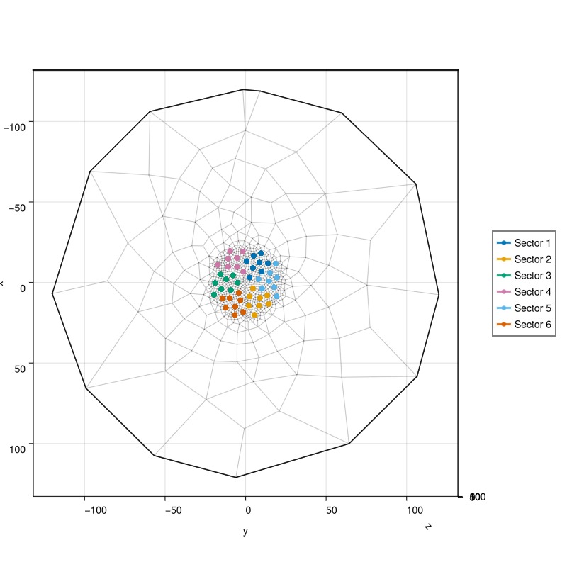
Set up reservoir simulator
We configure the simulator with specific tolerances and timestep controls to handle the challenging thermal transients in the BTES system. Since almost all of the challenging dynamics occurs in the wellbores, we also add a "preconditioning" strategy that starts each timestep by solving the well equations with fixed reservoir conditions.
simulator, config = setup_reservoir_simulator(case;
    presolve_wells = true,
    tol_cnv = 1e-2,
    tol_mb = 1e-6,
    tol_cnve_well = Inf,
    inc_tol_dT = 1e-2,
    timesteps = :auto,
    initial_dt = 5.0,
    target_its = 10,
    relaxation = true);
The transition from charging to discharging creates a thermal shock that is numerically challenging for the nonlinear solver. We use a specialized timestep selector that reduces the timestep to 5 seconds during control changes to maintain numerical stability and convergence.
sel = JutulDarcy.ControlChangeTimestepSelector(
    case.model, 0.0, convert_to_si(5.0, :second))
push!(config[:timestep_selectors], sel)
config[:timestep_max_decrease] = 1e-6;
Simulate the BTES system
Run the full 4-year simulation with the configured solver settings.
Note that this simulation can take a few minutes to run. Setting info_level = 0 will show a progress bar while the simulation runs.`
results = simulate_reservoir(case;
simulator=simulator, config=config, info_level=0);
Jutul: Simulating 4 years, 43.2 minutes as 109 report steps
╭────────────────┬───────────┬───────────────┬─────────────╮
│ Iteration type │ Avg/step │ Avg/ministep │ Total │
│ │ 109 steps │ 859 ministeps │ (wasted) │
├────────────────┼───────────┼───────────────┼─────────────┤
│ Newton │ 66.8807 │ 8.48661 │ 7290 (105) │
│ Linearization │ 74.7615 │ 9.48661 │ 8149 (112) │
│ Linear solver │ 185.954 │ 23.596 │ 20269 (105) │
│ Precond apply │ 371.908 │ 47.1921 │ 40538 (210) │
╰────────────────┴───────────┴───────────────┴─────────────╯
╭───────────────┬──────────┬────────────┬───────────╮
│ Timing type │ Each │ Relative │ Total │
│ │ ms │ Percentage │ s │
├───────────────┼──────────┼────────────┼───────────┤
│ Properties │ 3.7308 │ 2.07 % │ 27.1977 │
│ Equations │ 21.0195 │ 13.05 % │ 171.2876 │
│ Assembly │ 9.4882 │ 5.89 % │ 77.3192 │
│ Linear solve │ 3.5374 │ 1.96 % │ 25.7875 │
│ Linear setup │ 34.8421 │ 19.35 % │ 253.9992 │
│ Precond apply │ 2.2422 │ 6.92 % │ 90.8937 │
│ Update │ 1.5260 │ 0.85 % │ 11.1247 │
│ Convergence │ 3.5750 │ 2.22 % │ 29.1328 │
│ Input/Output │ 0.1384 │ 0.01 % │ 0.1189 │
│ Other │ 85.8658 │ 47.68 % │ 625.9620 │
├───────────────┼──────────┼────────────┼───────────┤
│ Total │ 180.0855 │ 100.00 % │ 1312.8233 │
╰───────────────┴──────────┴────────────┴───────────╯Interactive visualization of results
We first plot the final temperature distribution in the reservoir and well performance over time. The reservoir plot shows the thermal plumes developed around each well sector, while the well results show the temperature and flow rate evolution throughout the simulation.
plot_reservoir(case.model, results.states;
well_fontsize = 0, key = :Temperature, step = length(case.dt),
colormap = :seaborn_icefire_gradient)

plot_well_results(results.wells, field = :temperature)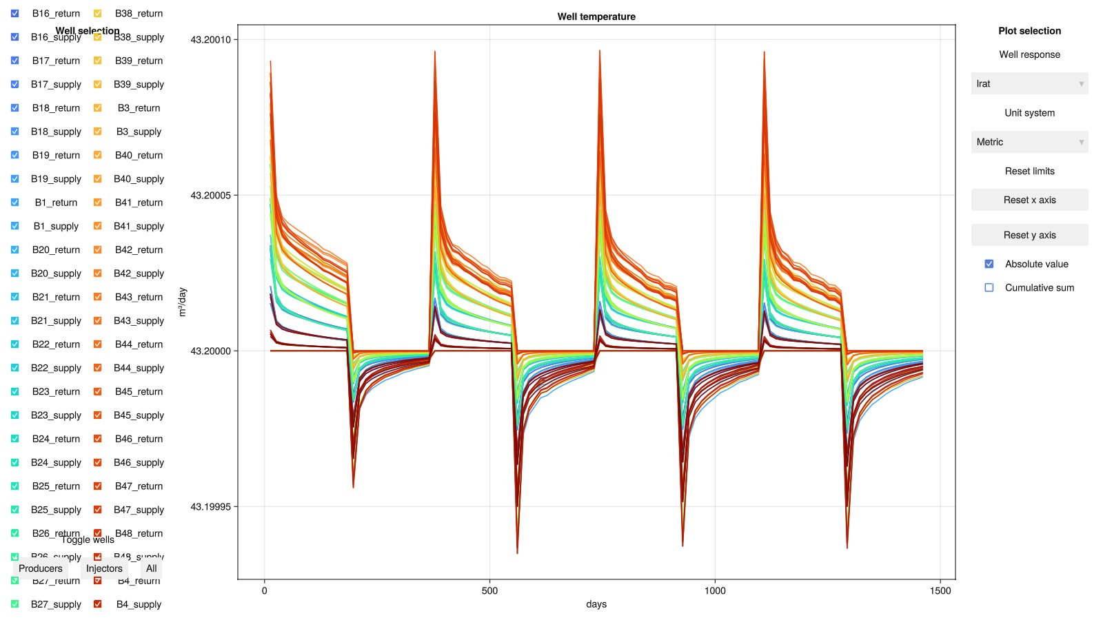
Temperature evolution in the reservoir
Next, we visualize how thermal energy storage develops in the subsurface over time. We examine the temperature distribution after each of the four charging cycles to see how the thermal plume grows. For better visualization, we only display cells below 50 m depth with temperatures above 15°C (warmer than the natural ground temperature).
using Dates
charge_end = Dates.monthname.(case.input_data[:timestamps]) .== "October" .&&
    Dates.day.(case.input_data[:timestamps]) .== 1
steps = findall(charge_end)
fig = Figure(size = (1000, 750))
geo = tpfv_geometry(msh)
bottom = geo.cell_centroids[3,:] .>= 50.0
T_min, T_max = Inf, -Inf
for (sno, step) in enumerate(steps)
    ax_sno = Axis3(fig[(sno-1)÷2+1, (sno-1)%2+1];
    limits = (-50, 50, -50, 50, 40, 125),
    title = "Charge $sno", zreversed = true, aspect = :data)
    T = convert_from_si.(results.states[step][:Temperature], :Celsius)
    cells = bottom .& (T .>= 15.0)
    global T_min = min(T_min, minimum(T[cells]))
    global T_max = max(T_max, maximum(T[cells]))
    plot_cell_data!(ax_sno, msh, T; cells = cells, colormap = :seaborn_icefire_gradient)
    hidedecorations!(ax_sno)
end
Colorbar(fig[1:2, 3];
colormap = :seaborn_icefire_gradient, colorrange = (T_min, T_max),
label = "T ≥ 15.0 °C", vertical = true)
fig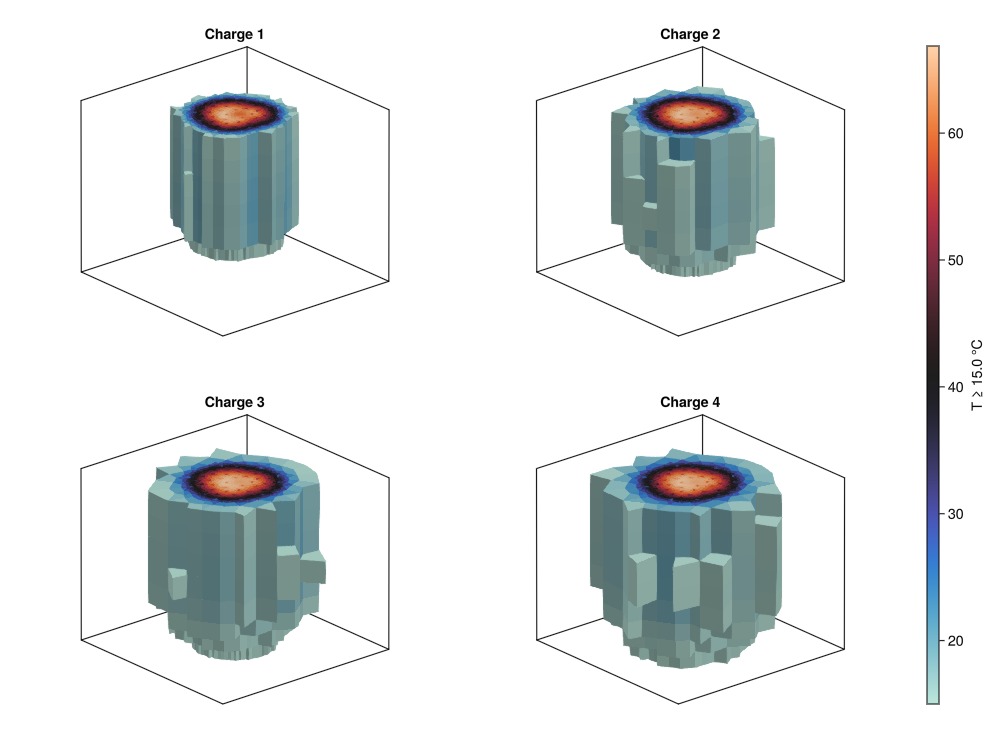
Temperature evolution within the boreholes
Understanding the temperature profiles within individual boreholes is crucial for BTES system design. We analyze how temperature varies with depth along the wellbore during both charging and discharging phases. This information can help determine optimal well depth, number of wells needed, and the most effective series/parallel coupling configuration for a given thermal storage capacity requirement.
To this end, we define a utility function to plot temperature evolution in a BTES sector. This function visualizes temperature as a function of well depth for all wells in a given sector at specified timesteps, helping to understand thermal propagation through the wellbore network.
function plot_btes_temperature(ax, sector, timesteps)
    colors = cgrad(:ice, length(timesteps), categorical = true)
    msh = physical_representation(reservoir_model(case.model).data_domain)
    geo = tpfv_geometry(msh)
    time = convert_from_si.(cumsum(case.dt), :day)
    out = []
    for (sno, step) in enumerate(timesteps)
        label = String("$(round((time[step]),digits=1)) days")
        for (wno, well) in enumerate(sectors[Symbol("S$sector")])
            lbl = wno == 1 ? label : nothing
            T = results.result.states[step][well][:Temperature]
            T = convert_from_si.(T, :Celsius)
            wm = case.model.models[well]
            num_nodes = length(wm.domain.representation.perforations.reservoir)
            plot_mswell_values!(ax, case.model, well, T;
            nodes = 1:num_nodes, geo = geo, color = colors[sno], linewidth = 6, label = lbl)
        end
    end
end

fig = Figure(size = (1000, 750))
sector = 1
sectors = case.input_data[:sectors]
Dict{Any, Any} with 6 entries:
:S6 => [:B1_supply, :B1_return, :B9_supply, :B9_return, :B14_supply, :B14_ret…
:S4 => [:B3_supply, :B3_return, :B8_supply, :B8_return, :B16_supply, :B16_ret…
:S2 => [:B2_supply, :B2_return, :B7_supply, :B7_return, :B10_supply, :B10_ret…
:S1 => [:B4_supply, :B4_return, :B12_supply, :B12_return, :B20_supply, :B20_r…
:S5 => [:B6_supply, :B6_return, :B11_supply, :B11_return, :B19_supply, :B19_r…
:S3 => [:B5_supply, :B5_return, :B13_supply, :B13_return, :B18_supply, :B18_r…Temperature evolution during the first charging cycle
We first visualize how thermal energy propagates through the wellbore network as hot water flows from the innermost to the outermost well in the sector.
well = sectors[Symbol("S$sector")][1]
T_ch = convert_to_si(90.0, :Celsius)
is_charge = [f[:Facility].control[well].temperature == T_ch for f in case.forces]
stop = findfirst(diff(is_charge) .< 0)
ax = Axis(fig[1, 1]; title = "Temperature evolution, sector $sector (charging)",
xlabel = "T [°C]", ylabel = "Depth [m]", yreversed = true)
plot_btes_temperature(ax, sector, 1:stop)
Legend(fig[1,2], ax; fontsize = 20)Makie.Legend()Temperature evolution during the first discharging cycle
Next, we show how stored thermal energy is extracted as flow direction reverses, with water flowing from the outermost to the innermost well.
well = sectors[Symbol("S$sector")][end-1]
T_dch = convert_to_si(10.0, :Celsius)
is_discharge = [f[:Facility].control[well].temperature == T_dch for f in case.forces]
start = findfirst(diff(is_discharge) .> 0)+1
stop = findfirst(diff(is_discharge) .< 0)
ax = Axis(fig[2, 1]; title = "Temperature evolution, sector $sector (discharging)",
xlabel = "T [°C]", ylabel = "Depth [m]", yreversed = true)
plot_btes_temperature(ax, sector, start:stop)
Legend(fig[2,2], ax; fontsize = 20)

fig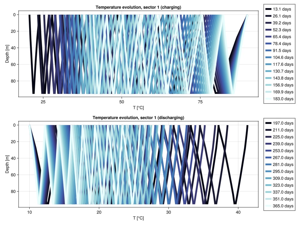
Example on GitHub
If you would like to run this example yourself, it can be downloaded from the Fimbul.jl GitHub repository as a script.
This example took 1412.066400643 seconds to complete.This page was generated using Literate.jl.