Deep coaxial borehole heat exchanger (BHE) demo

This example demonstrates simulation and analysis of geothermal energy production from a deep coaxial closed-loop well. The well is defined by a general trajectory (m×3 matrix) and consists of to concentric pipes: an inner supply pipe and an outer return annulus.

We explore three scenarios:

1. Homogeneous reservoir: A single uniform layer to establish a baseline, comparing injection into the inner pipe vs. the outer annulus.

2. Layered reservoir: Four distinct geological layers (clay, sandstone, granite, sandstone) with varying thermal conductivities to highlight the effect of heterogeneity on heat extraction.

3. Inner pipe conductivity study: Homogeneous reservoir with varying inner pipe wall thermal conductivity (from 0 to 4× default) to demonstrate the effect of heat loss between supply and return pipes.

Add required modules to namespace

using Jutul, JutulDarcy, Fimbul
using HYPRE
using GLMakie
using Statistics

Useful SI units

meter, hour, watt, Kelvin, joule, kilogram = si_units(
    :meter, :hour, :watt, :Kelvin, :joule, :kilogram);

Common parameters

All scenarios share the same well trajectory, flow rate, injection temperature, simulation duration, and mesh settings.

well_trajectory = [
    0.0  0.0     0.0;
    0.0  0.0  2500.0;
]
base_args = (
    well_trajectory = well_trajectory,
    rate = 25meter^3/hour,
    temperature_inj = convert_to_si(25.0, :Celsius),
    num_years = 10,
    report_interval = si_unit(:year),
    hxy_min = 2.5,
    mesh_args = (offset = 250.0, offset_rel = missing),
);

Simulator helper

A reusable function to run any case with consistent solver settings.

function run_case(case)
    sim, cfg = setup_reservoir_simulator(case;
        output_substates = true,
        info_level = 0,
        initial_dt = 120.0,
        presolve_wells = true,
        relaxation = true)
    sel = VariableChangeTimestepSelector(:Temperature, 5.0;
        relative = false, model = :Reservoir)
    push!(cfg[:timestep_selectors], sel)
    sel = VariableChangeTimestepSelector(:Temperature, 5.0;
        relative = false, model = :CoaxialWell_supply)
    push!(cfg[:timestep_selectors], sel)
    return simulate_reservoir(case; simulator = sim, config = cfg)
end

run_case (generic function with 1 method)

Scenario 1 – Homogeneous reservoir

A single uniform reservoir from the surface to 3000 m depth with constant rock properties. We compare two flow configurations: injection into the inner pipe vs. the outer annulus.

homogeneous_args = (;
    base_args...,
    depths = [0.0, 2550.0, 3000.0],
    permeability = [1e-2, 1e-2]*si_unit(:darcy),
    porosity = [0.01, 0.01],
    rock_thermal_conductivity = [2.5, 2.5]*watt/(meter*Kelvin),
    rock_heat_capacity = [900, 900]*joule/(kilogram*Kelvin),
    rock_density = [2600, 2600]*kilogram/meter^3,
);

case_hom_inner = coaxial_bhe(; inject_into = :inner, homogeneous_args...);
case_hom_outer = coaxial_bhe(; inject_into = :outer, homogeneous_args...);

Inspect mesh and well

msh_hom = physical_representation(reservoir_model(case_hom_inner.model).data_domain)
fig = Figure(size = (800, 800))
ax = Axis3(fig[1, 1]; zreversed = true, perspectiveness = 0.5, aspect = (1, 1, 4),
    title = "Homogeneous reservoir – mesh")
Jutul.plot_mesh_edges!(ax, msh_hom, alpha = 0.2)
wells = get_model_wells(case_hom_inner.model)
plot_well!(ax, msh_hom, wells[:CoaxialWell_supply]; fontsize=0.0)

fig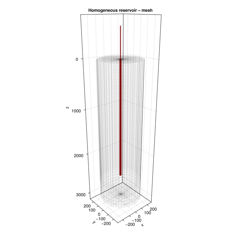

Simulate

results_hom_inner = run_case(case_hom_inner);
results_hom_outer = run_case(case_hom_outer);

Jutul: Simulating 9 years, 52.12 weeks as 12 report steps
╭────────────────┬──────────┬──────────────┬──────────╮
│ Iteration type │ Avg/step │ Avg/ministep │    Total │
│                │ 12 steps │ 42 ministeps │ (wasted) │
├────────────────┼──────────┼──────────────┼──────────┤
│ Newton         │  6.08333 │       1.7381 │   73 (0) │
│ Linearization  │  9.58333 │       2.7381 │  115 (0) │
│ Linear solver  │     22.0 │      6.28571 │  264 (0) │
│ Precond apply  │     44.0 │      12.5714 │  528 (0) │
╰────────────────┴──────────┴──────────────┴──────────╯
╭───────────────┬──────────┬────────────┬─────────╮
│ Timing type   │     Each │   Relative │   Total │
│               │       ms │ Percentage │       s │
├───────────────┼──────────┼────────────┼─────────┤
│ Properties    │   6.6000 │     1.31 % │  0.4818 │
│ Equations     │  93.4493 │    29.15 % │ 10.7467 │
│ Assembly      │   8.9064 │     2.78 % │  1.0242 │
│ Linear solve  │  20.4033 │     4.04 % │  1.4894 │
│ Linear setup  │  88.0041 │    17.43 % │  6.4243 │
│ Precond apply │   7.4228 │    10.63 % │  3.9193 │
│ Update        │   2.9803 │     0.59 % │  0.2176 │
│ Convergence   │   9.0296 │     2.82 % │  1.0384 │
│ Input/Output  │   0.8341 │     0.10 % │  0.0350 │
│ Other         │ 157.3186 │    31.16 % │ 11.4843 │
├───────────────┼──────────┼────────────┼─────────┤
│ Total         │ 504.9447 │   100.00 % │ 36.8610 │
╰───────────────┴──────────┴────────────┴─────────╯
Jutul: Simulating 9 years, 52.12 weeks as 12 report steps
╭────────────────┬──────────┬──────────────┬──────────╮
│ Iteration type │ Avg/step │ Avg/ministep │    Total │
│                │ 12 steps │ 40 ministeps │ (wasted) │
├────────────────┼──────────┼──────────────┼──────────┤
│ Newton         │      6.0 │          1.8 │   72 (0) │
│ Linearization  │  9.33333 │          2.8 │  112 (0) │
│ Linear solver  │     22.5 │         6.75 │  270 (0) │
│ Precond apply  │     45.0 │         13.5 │  540 (0) │
╰────────────────┴──────────┴──────────────┴──────────╯
╭───────────────┬──────────┬────────────┬─────────╮
│ Timing type   │     Each │   Relative │   Total │
│               │       ms │ Percentage │       s │
├───────────────┼──────────┼────────────┼─────────┤
│ Properties    │   6.6394 │     1.93 % │  0.4780 │
│ Equations     │  92.3085 │    41.67 % │ 10.3385 │
│ Assembly      │   7.0819 │     3.20 % │  0.7932 │
│ Linear solve  │  18.2936 │     5.31 % │  1.3171 │
│ Linear setup  │  99.5672 │    28.89 % │  7.1688 │
│ Precond apply │   7.4635 │    16.24 % │  4.0303 │
│ Update        │   2.1123 │     0.61 % │  0.1521 │
│ Convergence   │   1.1375 │     0.51 % │  0.1274 │
│ Input/Output  │   0.2071 │     0.03 % │  0.0083 │
│ Other         │   5.5449 │     1.61 % │  0.3992 │
├───────────────┼──────────┼────────────┼─────────┤
│ Total         │ 344.6256 │   100.00 % │ 24.8130 │
╰───────────────┴──────────┴────────────┴─────────╯

Thermal depletion – inner vs. outer injection

Visualize the temperature change (ΔT) from initial conditions in the reservoir after 10 years for each flow configuration. A quadrant is cut away for better visibility.

fig_cmp = Figure(size = (1200, 800))
for (i, (results, case, label)) in enumerate(zip(
    [results_hom_inner, results_hom_outer],
    [case_hom_inner, case_hom_outer],
    ["Inject into inner", "Inject into outer"]))
    Δstates = JutulDarcy.delta_state(results.states, case.state0[:Reservoir])
    ax = Axis3(fig_cmp[1, i]; zreversed = true, perspectiveness = 0.5,
        aspect = (1, 1, 3), title = label)
    x = reservoir_model(case.model).data_domain[:cell_centroids]
    cell_mask = .!(x[1, :] .< 0.0 .&& x[2, :] .< 0.0)
    Jutul.plot_cell_data!(ax, msh_hom, Δstates[end][:Temperature];
        cells = cell_mask, colormap = :seaborn_icefire_gradient)
end
fig_cmp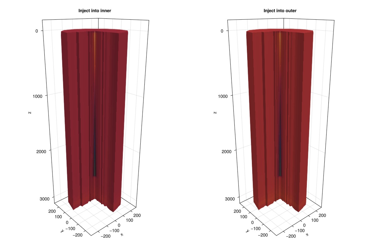

Well temperature profiles

Side-by-side comparison of temperature with depth for the two flow configurations. The black line shows the reservoir temperature at the perforated cells for reference. We see that the production temperature is higher for outer injection since temperature difference between injected fluid and reservoir is larger along the wellbore. We therefore use outer injection for the remaining scenarios in this demo.

fig_hom = Figure(size = (600, 600))
colors = cgrad(:BrBG_4, 4, categorical = true)[[1, 2, 4]]

for (i, (c, r, l)) in enumerate(zip(
    [results_hom_inner, results_hom_outer],
    [case_hom_inner, case_hom_outer],
    ["Injection in inner pipe", "Injection in outer annulus"]))

    ax = Axis(fig_hom[i, 1];
        title = l,
        xlabel = "Temperature (°C)",
        ylabel = "Depth (m)",
        xticks = 0:5:100,
        yreversed = true)

    well = r.model.models[:CoaxialWell_supply].data_domain
    T_well = convert_from_si.(
        c.result.states[end][:CoaxialWell_supply][:Temperature], :Celsius)
    tags = well[:tag] |> unique |> collect

    for (j, tag) in enumerate(tags)
        name = titlecase(replace(string(tag), "_" => " "))
        cells = well[:tag] .== tag
        Tn = T_well[cells]
        zn = well[:cell_centroids][3, cells]
        lines!(ax, Tn, zn; color = colors[j], linewidth = 4, label = name)
    end
    reservoir_cells = well.representation.perforations.reservoir
    T_reservoir = convert_from_si.(
        c.result.states[end][:Reservoir][:Temperature], :Celsius)
    T_reservoir_perf = T_reservoir[reservoir_cells]
    zn_reservoir = r.model.models[:Reservoir].data_domain[:cell_centroids][3, reservoir_cells]
    lines!(ax, T_reservoir_perf, zn_reservoir; color = :black, linewidth = 2, label = "Reservoir")
    axislegend(ax; position = :rt)
end
linkaxes!(filter(c -> c isa Axis, fig_hom.content)...)
fig_hom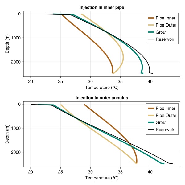

Scenario 2 – Layered reservoir

Four geological layers span the same 0–3000 m interval, each with distinct thermal and hydraulic properties. The layers are (from top to bottom):

• Clay (0–250 m): low conductivity (1.0 W/(m·K)), low permeability

• Sandstone (250–750 m): moderate conductivity (2.0 W/(m·K)), higher permeability

• Granite (750–1250 m): high conductivity (4.0 W/(m·K)), very low permeability

• Sandstone (1250–3000 m): moderate conductivity (2.0 W/(m·K)), higher permeability

The thermal conductivity contrast is somewhat exaggerated to clearly show the impact of layering on the well temperature profiles.

layered_args = (;
    base_args...,
    depths = [0.0, 250.0, 750.0, 1250.0, 3000.0],
    permeability  = [1e-3, 1e-1, 1e-4, 1e-1]*si_unit(:darcy),
    porosity      = [0.15, 0.20, 0.01, 0.20],
    rock_thermal_conductivity = [1.0, 2.0, 4.0, 2.0]*watt/(meter*Kelvin),
    rock_heat_capacity = [800, 900, 950, 900]*joule/(kilogram*Kelvin),
    rock_density       = [2650, 2600, 2580, 2600]*kilogram/meter^3,
);

case_layered = coaxial_bhe(; inject_into = :outer, layered_args...);

Plot reservoir properties

The interactive viewer shows how conductivity and other properties vary with depth across the four layers.

plot_reservoir(case_layered.model)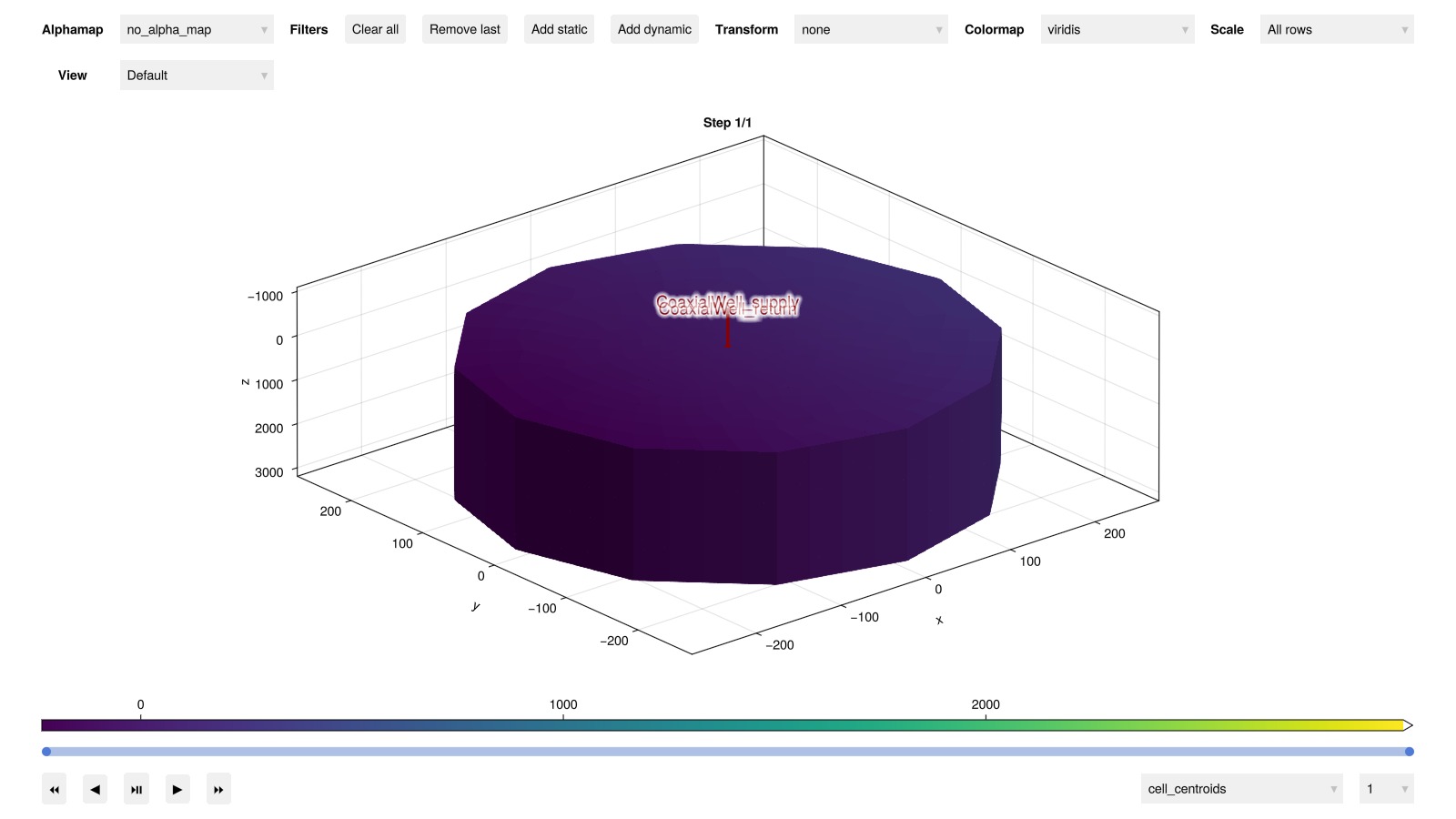

Simulate

results_layered = run_case(case_layered);

Jutul: Simulating 9 years, 52.12 weeks as 12 report steps
╭────────────────┬──────────┬──────────────┬──────────╮
│ Iteration type │ Avg/step │ Avg/ministep │    Total │
│                │ 12 steps │ 40 ministeps │ (wasted) │
├────────────────┼──────────┼──────────────┼──────────┤
│ Newton         │     6.25 │        1.875 │   75 (0) │
│ Linearization  │  9.58333 │        2.875 │  115 (0) │
│ Linear solver  │  23.0833 │        6.925 │  277 (0) │
│ Precond apply  │  46.1667 │        13.85 │  554 (0) │
╰────────────────┴──────────┴──────────────┴──────────╯
╭───────────────┬──────────┬────────────┬─────────╮
│ Timing type   │     Each │   Relative │   Total │
│               │       ms │ Percentage │       s │
├───────────────┼──────────┼────────────┼─────────┤
│ Properties    │   7.1768 │     1.96 % │  0.5383 │
│ Equations     │ 101.8513 │    42.62 % │ 11.7129 │
│ Assembly      │   7.9773 │     3.34 % │  0.9174 │
│ Linear solve  │  20.1052 │     5.49 % │  1.5079 │
│ Linear setup  │ 100.1878 │    27.34 % │  7.5141 │
│ Precond apply │   8.3295 │    16.79 % │  4.6145 │
│ Update        │   2.2622 │     0.62 % │  0.1697 │
│ Convergence   │   1.2356 │     0.52 % │  0.1421 │
│ Input/Output  │   0.2323 │     0.03 % │  0.0093 │
│ Other         │   4.7281 │     1.29 % │  0.3546 │
├───────────────┼──────────┼────────────┼─────────┤
│ Total         │ 366.4095 │   100.00 % │ 27.4807 │
╰───────────────┴──────────┴────────────┴─────────╯

Compare homogeneous vs layered well temperature profiles

The homogeneous result (outer injection) is shown alongside the layered result to emphasize how layer contrasts in thermal conductivity affect the temperature distribution along the wellbore.

fig_layers = Figure(size = (600, 600))

for (i, (results, case, label)) in enumerate(zip(
    [results_hom_outer, results_layered],
    [case_hom_outer, case_layered],
    ["Homogeneous", "Layered (clay / sandstone / granite / sandstone)"]))

    ax = Axis(fig_layers[i, 1];
        title = label,
        xlabel = "Temperature (°C)",
        ylabel = "Depth (m)",
        xticks = 0:5:100,
        yreversed = true)

    well = case.model.models[:CoaxialWell_supply].data_domain
    T_well = convert_from_si.(
        results.result.states[end][:CoaxialWell_supply][:Temperature], :Celsius)
    tags = well[:tag] |> unique |> collect

    for (j, tag) in enumerate(tags)
        name = titlecase(replace(string(tag), "_" => " "))
        cells = well[:tag] .== tag
        Tn = T_well[cells]
        zn = well[:cell_centroids][3, cells]
        lines!(ax, Tn, zn; color = colors[j], linewidth = 4, label = name)
    end
    res_cells = well.representation.perforations.reservoir
    T_res = convert_from_si.(
        results.result.states[end][:Reservoir][:Temperature], :Celsius)
    T_res_perf = T_res[res_cells]
    zn_res = case.model.models[:Reservoir].data_domain[:cell_centroids][3, res_cells]
    lines!(ax, T_res_perf, zn_res; color = :black, linewidth = 2, label = "Reservoir")
    axislegend(ax; position = :rt)
end
linkaxes!(filter(c -> c isa Axis, fig_layers.content)...)
fig_layers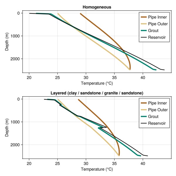

Scenario 3 – Effect of inner pipe wall thermal conductivity

Using the homogeneous reservoir with outer injection, we vary the inner pipe wall thermal conductivity from 0.0 (perfectly insulating inner pipe) to 4× the default value of 0.38 W/(m·K). A higher conductivity increases heat transfer between the supply and return pipes, causing more thermal short-circuiting and a lower production temperature.

λ_default = 0.38  # default inner pipe wall thermal conductivity [W/(m·K)]
λ_values = [0.0*λ_default, λ_default, 4.0*λ_default]
labels_λ = ["λ = 0.00", "λ = 0.38 (default)", "λ = 1.52"]

cases_λ = []
results_λ = []
for λ in λ_values
    case_i = coaxial_bhe(;
        inject_into = :outer,
        homogeneous_args...,
        well_args = (inner_pipe_thermal_conductivity = λ,
        outer_pipe_thermal_conductivity = λ_default, # keep outer pipe conductivity constant),
    ))
    push!(cases_λ, case_i)
    push!(results_λ, run_case(case_i))
end

Jutul: Simulating 9 years, 52.12 weeks as 12 report steps
╭────────────────┬──────────┬──────────────┬──────────╮
│ Iteration type │ Avg/step │ Avg/ministep │    Total │
│                │ 12 steps │ 54 ministeps │ (wasted) │
├────────────────┼──────────┼──────────────┼──────────┤
│ Newton         │  6.91667 │      1.53704 │   83 (0) │
│ Linearization  │  11.4167 │      2.53704 │  137 (0) │
│ Linear solver  │  20.3333 │      4.51852 │  244 (0) │
│ Precond apply  │  40.6667 │      9.03704 │  488 (0) │
╰────────────────┴──────────┴──────────────┴──────────╯
╭───────────────┬──────────┬────────────┬─────────╮
│ Timing type   │     Each │   Relative │   Total │
│               │       ms │ Percentage │       s │
├───────────────┼──────────┼────────────┼─────────┤
│ Properties    │   6.6741 │     2.04 % │  0.5539 │
│ Equations     │  91.5879 │    46.20 % │ 12.5475 │
│ Assembly      │   7.4909 │     3.78 % │  1.0263 │
│ Linear solve  │  15.2031 │     4.65 % │  1.2619 │
│ Linear setup  │  86.6318 │    26.47 % │  7.1904 │
│ Precond apply │   7.6116 │    13.68 % │  3.7145 │
│ Update        │   2.1043 │     0.64 % │  0.1747 │
│ Convergence   │   1.1441 │     0.58 % │  0.1567 │
│ Input/Output  │   0.1514 │     0.03 % │  0.0082 │
│ Other         │   6.3582 │     1.94 % │  0.5277 │
├───────────────┼──────────┼────────────┼─────────┤
│ Total         │ 327.2511 │   100.00 % │ 27.1618 │
╰───────────────┴──────────┴────────────┴─────────╯
Jutul: Simulating 9 years, 52.12 weeks as 12 report steps
╭────────────────┬──────────┬──────────────┬──────────╮
│ Iteration type │ Avg/step │ Avg/ministep │    Total │
│                │ 12 steps │ 40 ministeps │ (wasted) │
├────────────────┼──────────┼──────────────┼──────────┤
│ Newton         │      6.0 │          1.8 │   72 (0) │
│ Linearization  │  9.33333 │          2.8 │  112 (0) │
│ Linear solver  │     22.5 │         6.75 │  270 (0) │
│ Precond apply  │     45.0 │         13.5 │  540 (0) │
╰────────────────┴──────────┴──────────────┴──────────╯
╭───────────────┬──────────┬────────────┬─────────╮
│ Timing type   │     Each │   Relative │   Total │
│               │       ms │ Percentage │       s │
├───────────────┼──────────┼────────────┼─────────┤
│ Properties    │   6.6947 │     2.01 % │  0.4820 │
│ Equations     │  91.2986 │    42.69 % │ 10.2254 │
│ Assembly      │   7.4121 │     3.47 % │  0.8302 │
│ Linear solve  │  18.8320 │     5.66 % │  1.3559 │
│ Linear setup  │  87.2085 │    26.21 % │  6.2790 │
│ Precond apply │   7.5667 │    17.06 % │  4.0860 │
│ Update        │   2.1060 │     0.63 % │  0.1516 │
│ Convergence   │   1.1609 │     0.54 % │  0.1300 │
│ Input/Output  │   1.7295 │     0.29 % │  0.0692 │
│ Other         │   4.7790 │     1.44 % │  0.3441 │
├───────────────┼──────────┼────────────┼─────────┤
│ Total         │ 332.6870 │   100.00 % │ 23.9535 │
╰───────────────┴──────────┴────────────┴─────────╯
Jutul: Simulating 9 years, 52.12 weeks as 12 report steps
╭────────────────┬──────────┬──────────────┬──────────╮
│ Iteration type │ Avg/step │ Avg/ministep │    Total │
│                │ 12 steps │ 35 ministeps │ (wasted) │
├────────────────┼──────────┼──────────────┼──────────┤
│ Newton         │  5.66667 │      1.94286 │   68 (0) │
│ Linearization  │  8.58333 │      2.94286 │  103 (0) │
│ Linear solver  │    24.75 │      8.48571 │  297 (0) │
│ Precond apply  │     49.5 │      16.9714 │  594 (0) │
╰────────────────┴──────────┴──────────────┴──────────╯
╭───────────────┬──────────┬────────────┬─────────╮
│ Timing type   │     Each │   Relative │   Total │
│               │       ms │ Percentage │       s │
├───────────────┼──────────┼────────────┼─────────┤
│ Properties    │   6.6293 │     1.95 % │  0.4508 │
│ Equations     │  91.4259 │    40.73 % │  9.4169 │
│ Assembly      │   7.3447 │     3.27 % │  0.7565 │
│ Linear solve  │  21.5198 │     6.33 % │  1.4633 │
│ Linear setup  │  87.4819 │    25.73 % │  5.9488 │
│ Precond apply │   7.5509 │    19.40 % │  4.4852 │
│ Update        │   2.1244 │     0.62 % │  0.1445 │
│ Convergence   │   1.1447 │     0.51 % │  0.1179 │
│ Input/Output  │   0.2241 │     0.03 % │  0.0078 │
│ Other         │   4.7967 │     1.41 % │  0.3262 │
├───────────────┼──────────┼────────────┼─────────┤
│ Total         │ 339.9691 │   100.00 % │ 23.1179 │
╰───────────────┴──────────┴────────────┴─────────╯

Well temperature profiles for different inner pipe conductivities

Each panel shows the temperature–depth profile for a given inner pipe conductivity value. Higher conductivity leads to more heat leakage from the hot return flow to the cold supply flow, reducing the net temperature gain at the surface.

fig_lambda = Figure(size = (600, 800))

for (i, (results, case, label)) in enumerate(
    zip(results_λ, cases_λ, labels_λ))

    ax = Axis(fig_lambda[i, 1];
        title = label,
        xlabel = "Temperature (°C)",
        ylabel = "Depth (m)",
        xticks = 0:5:100,
        yreversed = true)

    well = case.model.models[:CoaxialWell_supply].data_domain
    T_well = convert_from_si.(
        results.result.states[end][:CoaxialWell_supply][:Temperature], :Celsius)
    tags = well[:tag] |> unique |> collect

    for (j, tag) in enumerate(tags)
        name = titlecase(replace(string(tag), "_" => " "))
        cells = well[:tag] .== tag
        Tn = T_well[cells]
        zn = well[:cell_centroids][3, cells]
        lines!(ax, Tn, zn; color = colors[j], linewidth = 4, label = name)
    end
    res_cells = well.representation.perforations.reservoir
    T_res = convert_from_si.(
        results.result.states[end][:Reservoir][:Temperature], :Celsius)
    T_res_perf = T_res[res_cells]
    zn_res = case.model.models[:Reservoir].data_domain[:cell_centroids][3, res_cells]
    lines!(ax, T_res_perf, zn_res; color = :black, linewidth = 2, label = "Reservoir")
    if i < length(λ_values)
        hidexdecorations!(ax, grid = false)
    end
    i == 1 && axislegend(ax; position = :rt)
end
linkaxes!(filter(c -> c isa Axis, fig_lambda.content)...)
fig_lambda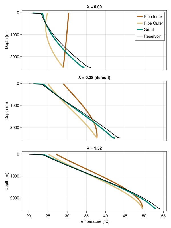

Power output over time

Compare the thermal power output at the production well for each inner pipe conductivity. Power is computed as mass flow rate × heat capacity × (production temperature − injection temperature). With a perfectly insulating inner pipe (λ = 0), the power output is almost thee times higher than the case with the highest conductivity.

fig_power = Figure(size = (800, 500))
ax_pwr = Axis(fig_power[1, 1];
    title = "Effect of inner pipe thermal conductivity",
    xlabel = "Time (years)",
    ylabel = "Power (MW)",
    limits = (nothing, (0.0, 0.4)),
    xticks = 0:1:10, yticks = 0:0.05:0.4)
colors_λ = Makie.wong_colors(length(λ_values))
T_inj = base_args.temperature_inj
for (i, (results, case, label)) in enumerate(zip(results_λ, cases_λ, labels_λ))
    T_prod = results.wells[:CoaxialWell_supply][:temperature]
    mrate = results.wells[:CoaxialWell_supply][:mass_rate]
    Cp = mean(reservoir_model(case.model).data_domain[:component_heat_capacity])
    power_mw = abs.(mrate .* Cp .* (T_prod .- T_inj)) ./ 1e6
    t_years = results.time ./ si_unit(:year)
    lines!(ax_pwr, t_years, power_mw; color = colors_λ[i], linewidth = 2, label = label)
end
axislegend(ax_pwr; position = :rt)
fig_power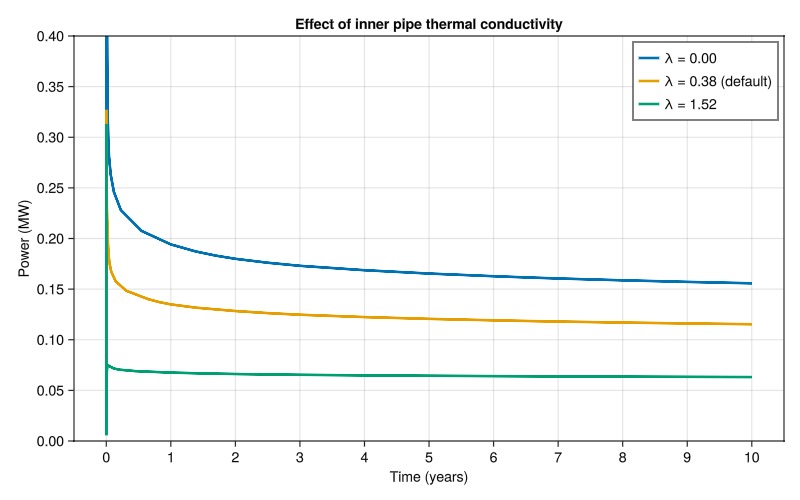

Example on GitHub

If you would like to run this example yourself, it can be downloaded from the Fimbul.jl GitHub repository as a script.

This example took 213.905319288 seconds to complete.

---

This page was generated using Literate.jl.