Analytical solutions for closed-loop geothermal wells

This example validates the numerical simulation of a closed-loop geothermal well system against analytical solutions for both U-tube and coaxial closed-loop configurations assuming fixed ground temperature. The validation demonstrates the accuracy of Fimbul's closed-loop well model implementation.

Add modules to namespace

julia

using Jutul, JutulDarcy, Fimbul
using HYPRE
using GLMakie

Useful SI units

julia

meter = si_unit(:meter)
kilogram = si_unit(:kilogram)
atm = si_unit(:atm)
second, day = si_units(:second, :day)
Kelvin, Joule, Watt = si_units(:kelvin, :joule, :watt)
darcy = si_unit(:darcy);

Problem parameters

We set up common parameters for both BTES configurations. These represent typical values for shallow geothermal systems.

Operational conditions

We inject fluid at 20.0 m^3/day and 80 °C temperature into the well, and assume a constant ground temperature of 10 °C.

julia

T_in = convert_to_si(80.0, :Celsius)   # Inlet temperature (supply fluid)
T_rock = convert_to_si(10.0, :Celsius) # Ground temperature (constant far-field)
Q = 20.0*meter^3/day                   # Volumetric flow rate through well

0.0002314814814814815

Fluid properties (water-based heat transfer fluid)

To enable comparison with analytical solutions, we use constant fluid properties.

julia

ρf = 988.1*kilogram/meter^3          # Fluid density at operating temperature
Cpf = 4184.0*Joule/(kilogram*Kelvin) # Specific heat capacity of fluid
λf = 0.6405*Watt/(meter*Kelvin)      # Thermal conductivity of fluid

0.6405

Rock formation properties (typical for sedimentary rock)

julia

ϕ = 0.01                            # Porosity (very low for compact rock)
K = 1e-3*darcy                      # Permeability (practically impermeable)
ρr = 2650.0*kilogram/meter^3        # Rock density
Cpr = 900.0*Joule/(kilogram*Kelvin) # Rock specific heat capacity
λr = 2.5*Watt/(meter*Kelvin)        # Rock thermal conductivity

2.5

Closed-loop installation materials

julia

ρg = 2000.0*kilogram/meter^3         # Grout density (cement/sand mixture)
Cpg = 1500.0*Joule/(kilogram*Kelvin) # Grout specific heat capacity
λg = 2.3*Watt/(meter*Kelvin)         # Grout thermal conductivity
λp = 0.38*Watt/(meter*Kelvin);       # Pipe wall thermal conductivity (HDPE)

Closed-loop configurations

We will consider two different closed-loop configurations: U-tube and coaxial.

U-tube configuration: The fluid flows down one pipe, makes a U-turn at the bottom, and returns to the surface through a parallel pipe. Both pipes are surrounded by grout within a single borehole.

Coaxial configuration: The fluid flows down an outer pipe and returns through an inner pipe concentrically located inside the outer pipe, or vice versa. This design allows for more compact installations.

In both configurations, the pipes are surrounded by grout material, which provides thermal contact with the rock formation while maintaining structural integrity of the borehole.

julia

L = 100.0*meter # Closed-loop well length (vertical depth)
cfg_u1 = ( # U-tube parameters
    closed_loop_type = :u1,
    radius_grout = 65e-3*meter,         # Borehole radius (grout outer boundary)
    radius_pipe = 16e-3*meter,          # Pipe outer radius (both supply/return)
    wall_thickness_pipe = 2.9e-3*meter, # Pipe wall thickness
    pipe_spacing = 60e-3*meter,         # Center-to-center distance between pipes
    pipe_thermal_conductivity = λp,     # Thermal conductivity of pipe material
)

cfg_coax = ( # Coaxial parameters
    closed_loop_type = :coaxial,
    radius_grout = 50e-3*meter,             # Borehole radius (grout outer boundary)
    radius_pipe_inner = 12e-3*meter,        # Inner pipe outer radius
    wall_thickness_pipe_inner = 3e-3*meter, # Inner pipe wall thickness
    radius_pipe_outer = 25e-3*meter,        # Outer pipe outer radius
    wall_thickness_pipe_outer = 4e-3*meter, # Outer pipe wall thickness
    inner_pipe_thermal_conductivity = λp,   # Inner pipe material conductivity
    outer_pipe_thermal_conductivity = λp    # Outer pipe material conductivity
);

Utility functions

We set up convenience functions to create closed-loop simulation cases and visualize results against analytical solutions. To mimic constant ground temperature, we set up a very large reservoir domain with a single cell in the horizontal directions.

julia

function setup_closed_loop_single( # Utility function to set up closed-loop simulation case
    type;          # Type of closed-loop geometry (:u1 or :coaxial)
    nz = 100,      # Number of cells in vertical direction
    n_step = 1,    # Number of time steps
    inlet = :outer # Inlet pipe for coaxial geometry (:outer or :inner
    )

    # Select well configuration based on geometry type
    if type == :u1
        well_args = cfg_u1
    elseif type == :coaxial
        well_args = cfg_coax
    else
        error("Unknown closed loop type: $type")
    end
    # Create computational domain
    dims = (1, 1, nz)
    Δ = (100000.0*dims[3]/L, 100000.0*dims[3]/L, L)
    msh = CartesianMesh(dims, Δ)
    reservoir = reservoir_domain(msh;
        rock_density = ρr,
        rock_heat_capacity = Cpr,
        rock_thermal_conductivity = λr,
        fluid_thermal_conductivity = λf,
        component_heat_capacity = Cpf,
        porosity = ϕ,
        permeability = K
    )
    # Set up closed-loop well
    wells = Fimbul.setup_vertical_btes_well(reservoir, 1, 1;
        name = :CL,
        well_args...,
        grouting_density = ρg,
        grouting_heat_capacity = Cpg,
        grouting_thermal_conductivity = λg
    )
    # Set up reservoir model
    sys = SinglePhaseSystem(AqueousPhase(), reference_density = ρf)
    model = setup_reservoir_model(reservoir, sys; wells = wells, thermal = true)
    # Set up controls and boundary conditions
    ctrl_inj = InjectorControl( # Injection control with fixed temperature
        TotalRateTarget(Q), [1.0],
        density=ρf, temperature=T_in)
    ctrl_prod = ProducerControl( # Production control with fixed BHP
        BottomHolePressureTarget(1.0*atm))
    geo = tpfv_geometry(msh)
    bc_cells = geo.boundary_neighbors
    domain = reservoir_model(model).data_domain
    bc = flow_boundary_condition( # Fixed pressure and temperature BCs
        bc_cells, domain, 5.0*atm, T_rock)
    # Set up forces and initial state
    if type == :coaxial && inlet == :outer # Coax with injection in outer pipe
        ctrl_supply = ctrl_prod
        ctrl_return = ctrl_inj
    else # Coax with injection in inner pipe or U1
        ctrl_supply = ctrl_inj
        ctrl_return = ctrl_prod
    end
    controls = Dict(
        :CL_supply => ctrl_supply,
        :CL_return => ctrl_return
    )
    forces = setup_reservoir_forces(model; control=controls, bc = bc)
    state0 = setup_reservoir_state( # Initialize with uniform pressure and temperature
        model; Pressure = 5*atm, Temperature = T_rock)
    # Set time large enough to ensure steady-state
    rg = well_args.radius_grout
    time = 5/4*2*rg*(ϕ*ρf*Cpf + (1 - ϕ)*ρr*Cpr)/(ϕ*λf + (1 - ϕ)*λr)*10
    dt = fill(time/n_step, n_step)
    # Create Jutul case
    case = JutulCase(model, dt, forces; state0 = state0)
    # Set up simulator with temperature-based timestep selector
    sim, cfg = setup_reservoir_simulator(
        case; initial_dt = 1.0);
    sel = VariableChangeTimestepSelector(:Temperature, 2.5;
        relative = false, model = :CL_supply)
    push!(cfg[:timestep_selectors], sel)

    return case, sim, cfg
end

function plot_closed_loop( # Utility function to plot closed-loop simulation results
    case, simulated, analytical; title = "Closed-loop temperature profiles"
    )

    # Create figure
    fig = Figure(size = (800, 600))
    ax = Axis(fig[1, 1],
        title = title,
        xlabel = "Temperature (°C)",
        ylabel = "Depth (m)",
        yreversed = true  # Surface at top, depth increases downward
    )
    # Extract numerical solution from final state
    well = case.model.models[:CL_supply].data_domain
    sim_temp = convert_from_si.(
        simulated.result.states[end][:CL_supply][:Temperature], :Celsius)
    za = collect(range(0, L, step=0.1)) # Analytical depth points
    section_handles = []
    solution_handles = []
    section_names = String[]
    solution_names = ["Analytical", "Fimbul"]
    # Plot results for each well section
    sections = last.(well[:section]) |> unique |> collect
    colors = cgrad(:BrBG_4, 4, categorical=true)[[1,2,4,3]]
    err_inf = -Inf
    for (i, section) in enumerate(sections)
        # Section name for printing
        name = titlecase(replace(string(section), "_" => " "))
        # Plot analytical solution
        Ta = convert_from_si.(analytical[section].(za), :Celsius)
        la = lines!(ax, Ta, za; color=colors[i], linewidth = 8, linestyle = :dash, label=name)
        # Plot numerical solution
        cells = last.(well[:section]) .== section
        Tn = sim_temp[cells]
        zn = well[:cell_centroids][3, cells]
        ln = lines!(ax, Tn, zn; color=colors[i], linewidth = 2)
        # Store handles and names for legend
        push!(section_handles, la)
        push!(section_names, name)
        if i == 1
           push!(solution_handles, la, ln)
        end
        # Compute maximum error in section
        Ta_n = convert_from_si.(analytical[section].(zn), :Celsius)
        e_inf = maximum(abs.(Tn .- Ta_n))
        err_inf = max(err_inf, e_inf)
    end
    # Add legend
    Legend(fig[1, 2], [section_handles, solution_handles], [section_names, solution_names],
        ["Sections", "Solutions"]; orientation = :vertical)

    return fig, err_inf

end;

Validate U-tube configuration

We set up and simulate a closed-loop system with U-tube geometry, and compare the numerical results against the analytical solution. This validates the implementation for the most common closed-loop configuration.

julia

case_u1, sim, cfg = setup_closed_loop_single(:u1; nz=125);
res_u1 = simulate_reservoir(case_u1; simulator = sim, config = cfg)

ReservoirSimResult with 1 entry:

  wells (2 present):
    :CL_supply
    :CL_return
    Results per well:
       :lrat => Vector{Float64} of size (1,)
       :wrat => Vector{Float64} of size (1,)
       :temperature => Vector{Float64} of size (1,)
       :control => Vector{Symbol} of size (1,)
       :Aqueous_mass_rate => Vector{Float64} of size (1,)
       :bhp => Vector{Float64} of size (1,)
       :wcut => Vector{Float64} of size (1,)
       :mass_rate => Vector{Float64} of size (1,)
       :rate => Vector{Float64} of size (1,)
       :mrat => Vector{Float64} of size (1,)

  states (Vector with 1 entries, reservoir variables for each state)
    :Pressure => Vector{Float64} of size (125,)
    :TotalMasses => Matrix{Float64} of size (1, 125)
    :TotalThermalEnergy => Vector{Float64} of size (125,)
    :FluidEnthalpy => Matrix{Float64} of size (1, 125)
    :Temperature => Vector{Float64} of size (125,)

  time (report time for each state)
     Vector{Float64} of length 1

  result (extended states, reports)
     SimResult with 1 entry

  extra
     Dict{Any, Any} with keys :simulator, :config

  Completed at Apr. 01 2026 17:56 after 27 seconds, 299 milliseconds, 779 microseconds.

Analytical solution

The function analytical_closed_loop_u1 computes the analytical steady-state solution for a vertical U-tube closed-loop system using the method of [2] as described in [3]. The function can be called with explicit parameters, but also has a convenience version that extracts parameters directly from the well model.

julia

analytical_u1 = Fimbul.analytical_closed_loop_u1(Q, T_in, T_rock,
    ρf, Cpf, case_u1.model.models[:CL_supply].data_domain)

Dict{Any, Any} with 4 entries:
  :grout_right => #temperature_grout_u1##2
  :pipe_left   => #temperature_closed_loop_pipe##14
  :pipe_right  => #temperature_closed_loop_pipe##16
  :grout_left  => #temperature_grout_u1##0

Plot comparison

The numerical solution agrees very well with the analytical solution.

julia

fig, err_inf = plot_closed_loop(case_u1, res_u1, analytical_u1;
    title = "U-tube temperature profiles")
println("Maximum error in U-tube configuration: $(round(err_inf, digits=3)) °C")
fig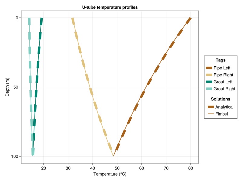

Validate coaxial configuration with outer pipe inlet

Next, we set up and simulate a closed-loop system with coaxial geometry, injecting fluid through the outer (annular) pipe, and compare the numerical results against the analytical solution.

julia

case_coax_outer, sim, cfg = setup_closed_loop_single(:coaxial; nz=125, inlet = :outer)
res_coax_outer = simulate_reservoir(case_coax_outer; simulator = sim, config = cfg, info_level = 0)

ReservoirSimResult with 1 entry:

  wells (2 present):
    :CL_supply
    :CL_return
    Results per well:
       :lrat => Vector{Float64} of size (1,)
       :wrat => Vector{Float64} of size (1,)
       :temperature => Vector{Float64} of size (1,)
       :control => Vector{Symbol} of size (1,)
       :Aqueous_mass_rate => Vector{Float64} of size (1,)
       :bhp => Vector{Float64} of size (1,)
       :wcut => Vector{Float64} of size (1,)
       :mass_rate => Vector{Float64} of size (1,)
       :rate => Vector{Float64} of size (1,)
       :mrat => Vector{Float64} of size (1,)

  states (Vector with 1 entries, reservoir variables for each state)
    :Pressure => Vector{Float64} of size (125,)
    :TotalMasses => Matrix{Float64} of size (1, 125)
    :TotalThermalEnergy => Vector{Float64} of size (125,)
    :FluidEnthalpy => Matrix{Float64} of size (1, 125)
    :Temperature => Vector{Float64} of size (125,)

  time (report time for each state)
     Vector{Float64} of length 1

  result (extended states, reports)
     SimResult with 1 entry

  extra
     Dict{Any, Any} with keys :simulator, :config

  Completed at Apr. 01 2026 17:57 after 2 seconds, 638 milliseconds, 312.5 microseconds.

Analytical solution

Following [3], we can also compute the analytical steady-state solution for coaxial closed-loop systems. This is implemented in analytical_closed_loop_coaxial. As or U-tube closed loops, this can be called with all parameters, or extract parameters from the well model. The function also accepts an inlet keyword argument to specify whether the fluid is injected through the outer or inner pipe.

julia

analytical_coax_outer = Fimbul.analytical_closed_loop_coaxial(Q, T_in, T_rock,
    ρf, Cpf, case_coax_outer.model.models[:CL_supply].data_domain; inlet = :outer)

Dict{Any, Any} with 3 entries:
  :pipe_inner => #temperature_closed_loop_pipe##16
  :grout      => #temperature_grout_coaxial##0
  :pipe_outer => #temperature_closed_loop_pipe##14

Plot comparison

Coaxial systems typically show different thermal behavior than U-tubes due to the closer thermal coupling between supply and return flows.

julia

fig, err_inf = plot_closed_loop(case_coax_outer, res_coax_outer, analytical_coax_outer;
    title = "Coaxial temperature profiles (outer inlet)")
println("Maximum error in coaxial outer inlet configuration: $(round(err_inf, digits=3)) °C")
fig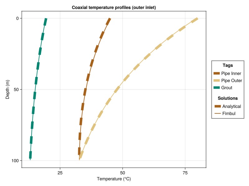

Validate coaxial configuration with inner pipe inlet

Finally, we validate the coaxial configuration with inner pipe inlet. This configuration is often preferred when storing heat, as the hot fluid is not exposed to the rock before it reaches the bottom of the well, ensuring a higher temperature difference along the entire wellbore, and consequently more heat storage.

julia

case_coax_inner, sim, cfg = setup_closed_loop_single(:coaxial; nz=125, inlet = :inner)
res_coax_inner = simulate_reservoir(case_coax_inner; simulator = sim, config = cfg, info_level = 0)

ReservoirSimResult with 1 entry:

  wells (2 present):
    :CL_supply
    :CL_return
    Results per well:
       :lrat => Vector{Float64} of size (1,)
       :wrat => Vector{Float64} of size (1,)
       :temperature => Vector{Float64} of size (1,)
       :control => Vector{Symbol} of size (1,)
       :Aqueous_mass_rate => Vector{Float64} of size (1,)
       :bhp => Vector{Float64} of size (1,)
       :wcut => Vector{Float64} of size (1,)
       :mass_rate => Vector{Float64} of size (1,)
       :rate => Vector{Float64} of size (1,)
       :mrat => Vector{Float64} of size (1,)

  states (Vector with 1 entries, reservoir variables for each state)
    :Pressure => Vector{Float64} of size (125,)
    :TotalMasses => Matrix{Float64} of size (1, 125)
    :TotalThermalEnergy => Vector{Float64} of size (125,)
    :FluidEnthalpy => Matrix{Float64} of size (1, 125)
    :Temperature => Vector{Float64} of size (125,)

  time (report time for each state)
     Vector{Float64} of length 1

  result (extended states, reports)
     SimResult with 1 entry

  extra
     Dict{Any, Any} with keys :simulator, :config

  Completed at Apr. 01 2026 17:57 after 3 seconds, 157 milliseconds, 866.4 microseconds.

Analytical solution

We compute the analytical solution for the coaxial configuration with inner pipe inlet.

julia

analytical_coax_inner = Fimbul.analytical_closed_loop_coaxial(Q, T_in, T_rock,
    ρf, Cpf, case_coax_inner.model.models[:CL_supply].data_domain; inlet = :inner)

Dict{Any, Any} with 3 entries:
  :pipe_inner => #temperature_closed_loop_pipe##14
  :grout      => #temperature_grout_coaxial##0
  :pipe_outer => #temperature_closed_loop_pipe##16

Plot comparison

julia

fig, err_inf = plot_closed_loop(case_coax_inner, res_coax_inner, analytical_coax_inner;
    title = "Coaxial temperature profiles (inner inlet)")
println("Maximum error in coaxial inner inlet configuration: $(round(err_inf, digits=3)) °C")
fig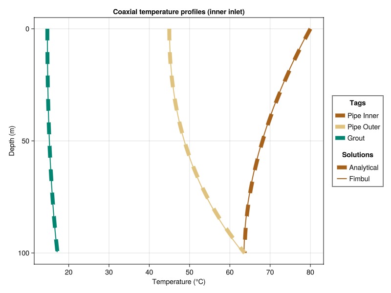

Example on GitHub

If you would like to run this example yourself, it can be downloaded from the Fimbul.jl GitHub repository as a script.

This example took 103.042113171 seconds to complete.

This page was generated using Literate.jl.

Analytical solutions for closed-loop geothermal wells ​

Problem parameters ​

Operational conditions ​

Fluid properties (water-based heat transfer fluid) ​

Rock formation properties (typical for sedimentary rock) ​

Closed-loop installation materials ​

Closed-loop configurations ​

Utility functions ​

Validate U-tube configuration ​

Analytical solution ​

Plot comparison ​

Validate coaxial configuration with outer pipe inlet ​

Analytical solution ​

Plot comparison ​

Validate coaxial configuration with inner pipe inlet ​

Analytical solution ​

Plot comparison ​

Example on GitHub ​

Analytical solutions for closed-loop geothermal wells

Problem parameters

Operational conditions

Fluid properties (water-based heat transfer fluid)

Rock formation properties (typical for sedimentary rock)

Closed-loop installation materials

Closed-loop configurations

Utility functions

Validate U-tube configuration

Analytical solution

Plot comparison

Validate coaxial configuration with outer pipe inlet

Analytical solution

Plot comparison

Validate coaxial configuration with inner pipe inlet

Analytical solution

Plot comparison

Example on GitHub