Geothermal energy production from a well doublet
ProductionThis example demonstrates how to simulate and visualize the production of geothermal energy from a doublet well system. The setup consists of a producer well that extracts hot water from the reservoir, and an injector well that reinjects produced water at a lower temperature.
Add required modules to namespace
using Jutul, JutulDarcy, Fimbul
using HYPRE
using GLMakie
Set up case
The injector and producer wells are placed 100 m apart at the top, and run parallel down to 800 m depth before they diverge to a distance of 1000 m at 2500 m depth.
case = geothermal_doublet();Inspect model
We first plot the computational mesh and wells. The mesh is refined around the wells in the horizontal plane and vertically in and near the target aquifer.
msh = physical_representation(reservoir_model(case.model).data_domain)
fig = Figure(size = (1200, 800))
ax = Axis3(fig[1, 1], zreversed = true, aspect = :data)
Jutul.plot_mesh_edges!(ax, msh, alpha = 1.0)
wells = get_model_wells(case.model)
for (k, w) in wells
    plot_well!(ax, msh, w)
end
fig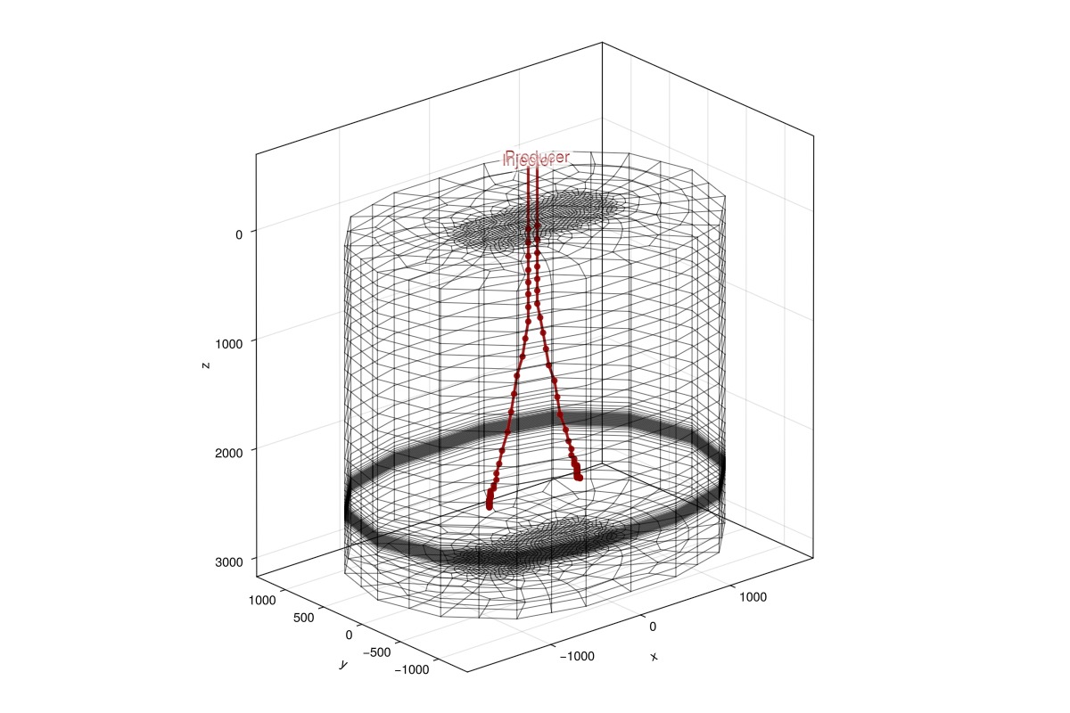
Plot reservoir properties
Next, we visualize the reservoir interactively.
plot_reservoir(case.model; aspect = :data)
Simulate geothermal energy production
We simulate the geothermal doublet for 200 years. The producer is set to produce at a rate of 300 m^3/hour with a lower BHP limit of 1 bar, while the injector is set to reinject the produced water, lowered to a temperature of 20 °C.
Note: this simulation can take a few minutes to run. Setting info_level = 0 will show a progress bar while the simulation runs.
results = simulate_reservoir(case; info_level = 0)ReservoirSimResult with 100 entries:
wells (2 present):
:Producer
:Injector
Results per well:
:lrat => Vector{Float64} of size (100,)
:wrat => Vector{Float64} of size (100,)
:temperature => Vector{Float64} of size (100,)
:control => Vector{Symbol} of size (100,)
:Aqueous_mass_rate => Vector{Float64} of size (100,)
:bhp => Vector{Float64} of size (100,)
:wcut => Vector{Float64} of size (100,)
:mass_rate => Vector{Float64} of size (100,)
:rate => Vector{Float64} of size (100,)
:mrat => Vector{Float64} of size (100,)
states (Vector with 100 entries, reservoir variables for each state)
:Pressure => Vector{Float64} of size (67032,)
:TotalMasses => Matrix{Float64} of size (1, 67032)
:TotalThermalEnergy => Vector{Float64} of size (67032,)
:FluidEnthalpy => Matrix{Float64} of size (1, 67032)
:Temperature => Vector{Float64} of size (67032,)
:PhaseMassDensities => Matrix{Float64} of size (1, 67032)
:RockInternalEnergy => Vector{Float64} of size (67032,)
:FluidInternalEnergy => Matrix{Float64} of size (1, 67032)
:PhaseViscosities => Matrix{Float64} of size (1, 67032)
time (report time for each state)
Vector{Float64} of length 100
result (extended states, reports)
SimResult with 100 entries
extra
Dict{Any, Any} with keys :simulator, :config
Completed at Jun. 20 2026 07:08 after 55 seconds, 995 milliseconds, 787.4 microseconds.Visualize results
We first plot the reservoir state interactively. You can notice how the cold front propagates from the injector well by filtering out high values.
plot_reservoir(case.model, results.states;
colormap = :seaborn_icefire_gradient, key = :Temperature, aspect = :data)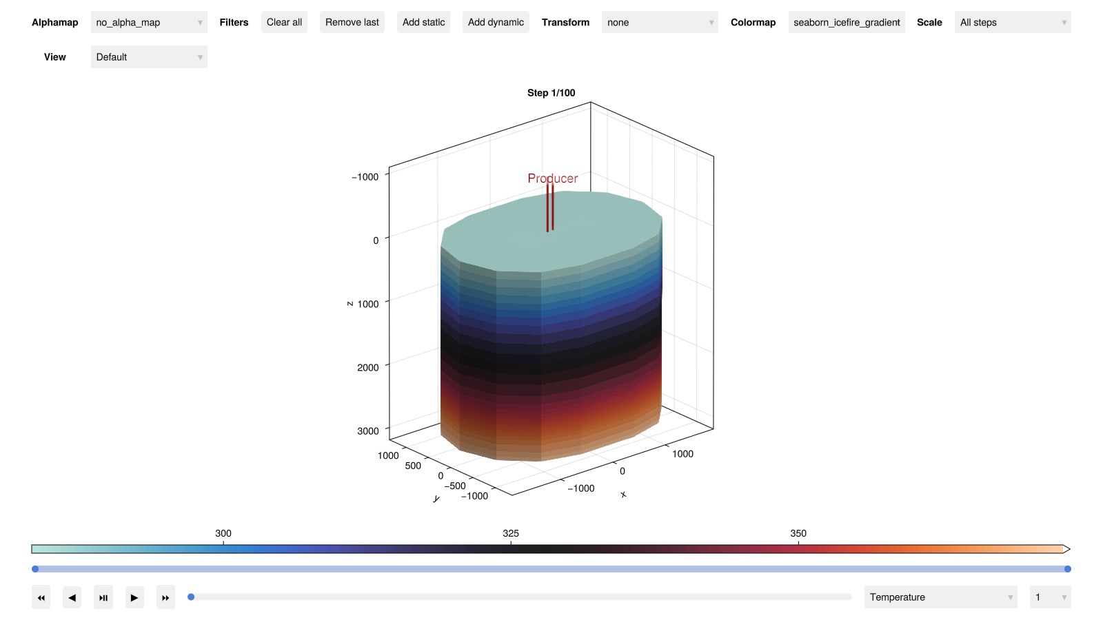
Plot well output
Next, we plot the well output to examine the production rates and temperatures.
plot_well_results(results.wells)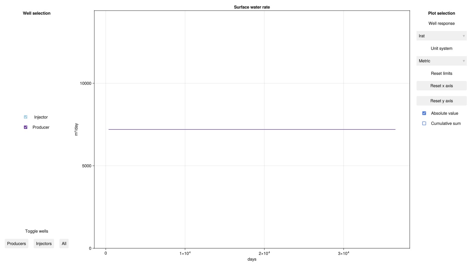
Well temperature evolution
For a more detailed analysis of the production temperature evolution, we plot the temperature inside the production well as a function of well depth for all 200 years of production. We also highlight the temperature at selected timesteps (7, 21, 65, and 200 years).
states = results.result.states
times = convert_from_si.(cumsum(case.dt), :year)
geo = tpfv_geometry(msh)

fig = Figure(size = (1200, 800))
ax = Axis(fig[1, 1], xlabel = "Temperature (°C)", ylabel = "Depth (m)", yreversed = true)
colors = cgrad(:seaborn_icefire_gradient, length(states), categorical = true);
Plot temperature profiles for all timesteps with transparency
for (n, state) in enumerate(states)
    T = convert_from_si.(state[:Producer][:Temperature], :Celsius)
    plot_mswell_values!(ax, case.model, :Producer, T;
    geo = geo, linewidth = 4, color = colors[n], alpha = 0.25)
end
Highlight selected timesteps with solid lines and labels
timesteps = [12, 25, 50, 100]
for n in timesteps
    T = convert_from_si.(states[n][:Producer][:Temperature], :Celsius)
    plot_mswell_values!(ax, case.model, :Producer, T;
    geo = geo, linewidth = 4, color = colors[n], label = "$(times[n]) years")
end
axislegend(ax; position = :lt, fontsize = 20)
fig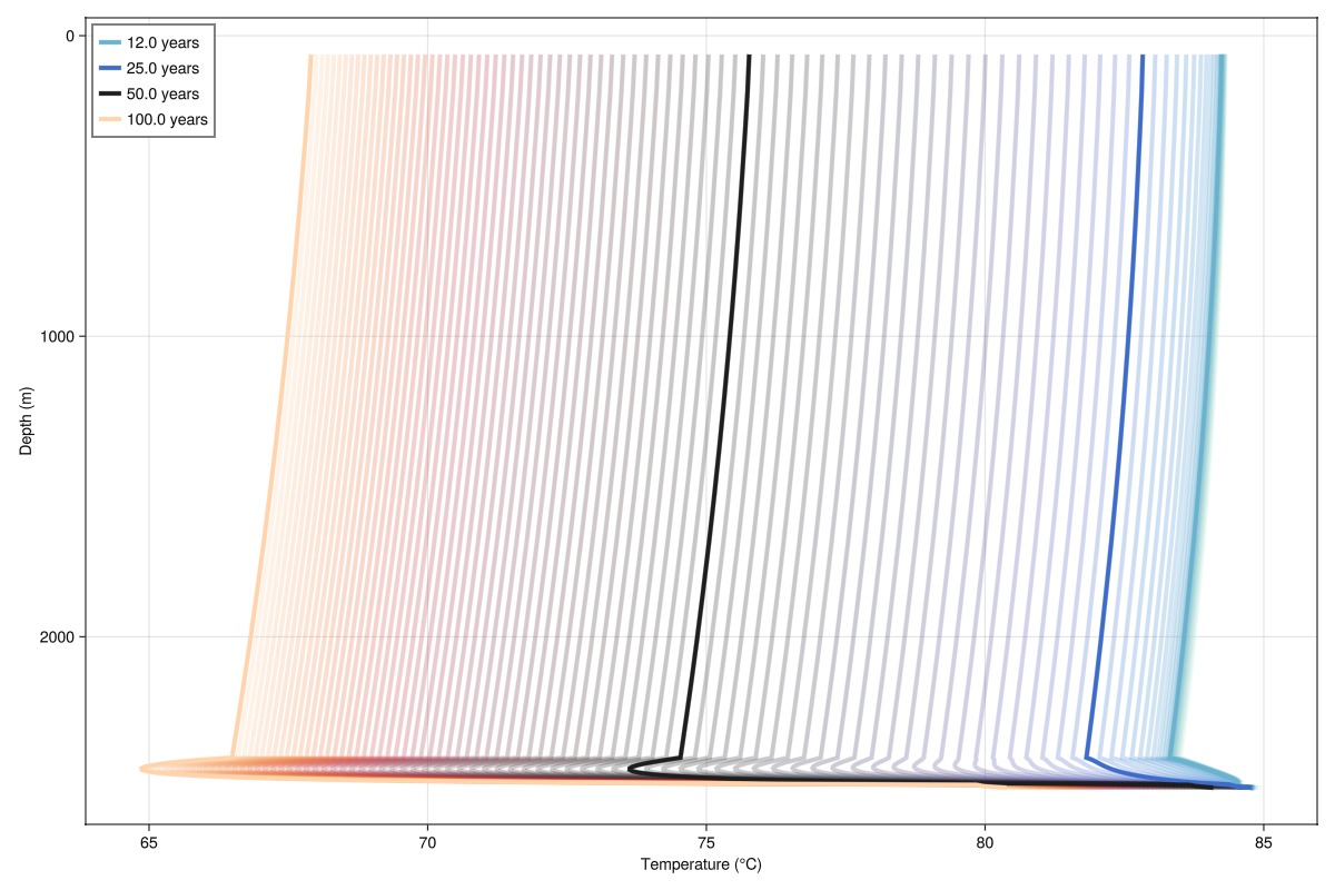
We can clearly see the footprint of the cold front in the aquifer (2400-2500 m depth) as it approaches the production well.
Reservoir state evolution
Another informative plot is the change in reservoir states over time. We compute the change in reservoir states from the initial state and plot the results interactively. The change in temperature is particularly interesting as it shows the evolution of the cold front in the aquifer
Δstates = JutulDarcy.delta_state(results.states, case.state0[:Reservoir])
plot_reservoir(case.model, Δstates;
colormap = :seaborn_icefire_gradient, key = :Temperature, aspect = :data)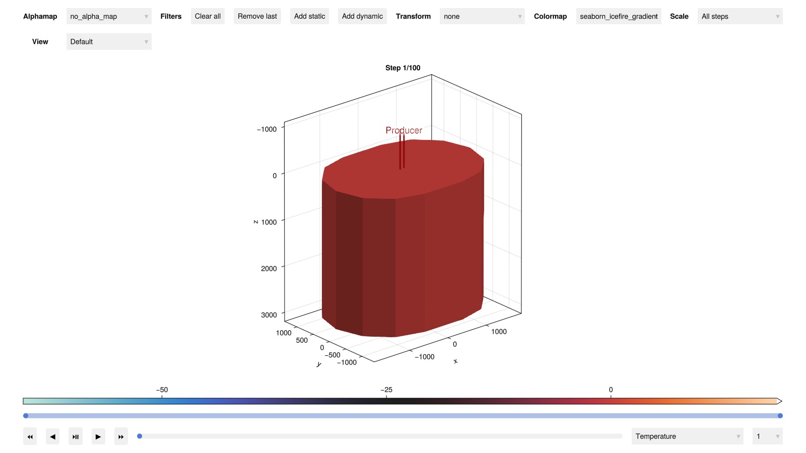
3D visualization of temperature changes
Finally, we plot the change in temperature at the same timesteps highlighted in the production well temperature above. We cut away parts of the model for better visualization. Define the temperature range and create a mask to cut away parts of the model
T_min = minimum(Δstates[end][:Temperature])
T_max = maximum(Δstates[1][:Temperature])
cells = geo.cell_centroids[1, :] .> -1000.0/2
cells = cells .&& geo.cell_centroids[2, :] .> 50.0
cells = cells .|| geo.cell_centroids[3, :] .> 2475.0;
Create subplots for each highlighted timestep
fig = Figure(size = (800, 800))
for (i, n) in enumerate(timesteps)
    ax_i = Axis3(fig[(i-1)÷2+1, (i-1)%2+1]; title = "$(times[n]) years",
    zreversed = true, elevation = pi/8, aspect = :data)

    ΔT = Δstates[n][:Temperature]

    plot_cell_data!(ax_i, msh, ΔT;
        cells = cells, colormap = :seaborn_icefire_gradient, colorrange = (T_min, T_max))
    plot_well!(ax_i, msh, wells[:Injector];
    color = :black, linewidth = 4, top_factor = 0.4, markersize = 0.0)
    plot_well!(ax_i, msh, wells[:Producer];
    color = :black, linewidth = 4, markersize = 0.0)
    hidedecorations!(ax_i)
end
Colorbar(fig[3, 1:2];
    colormap = :seaborn_icefire_gradient, colorrange = (T_min, T_max),
    label = "ΔT (°C)", vertical = false)
fig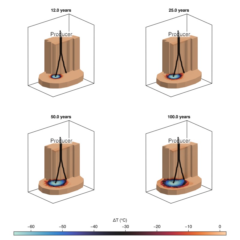
Example on GitHub
If you would like to run this example yourself, it can be downloaded from the Fimbul.jl GitHub repository as a script.
This example took 86.774715774 seconds to complete.This page was generated using Literate.jl.