Enhanced Geothermal System (EGS)

This example demonstrates simulation and analysis of energy production from an Enhanced Geothermal System (EGS). EGS technology enables geothermal energy extraction from hot dry rock formations where natural permeability is insufficient for fluid circulation.

This example exhibits issues with grid orientation effects, and will be updated when necessary flux discretization improvements are in place in JutulDarcy.

Add required modules to namespace

using Jutul, JutulDarcy, Fimbul # Core reservoir simulation framework
using HYPRE # High-performance linear solvers
using GLMakie # 3D visualization and plotting capabilities

Useful SI units

meter, day, watt = si_units(:meter, :day, :watt);
GWh = si_unit(:giga) * si_unit(:watt) * si_unit(:hour);

EGS setup

We consider an EGS system with one injection well and two production wells. The wells extend 2500 m vertically before continuing 1000 m horizontally. The horizontal sections are arranged in a triangular pattern, connected by a stimulated fracture network comprising multiple fractures intersecting the wells at right angles. Thermal energy is extracted by circulating cold water through the fracture network, which heats up by conduction from the surrounding rock matrix. To leverage buoyancy effects, the injection well is placed at a lower elevation than the production wells, forcing the colder (and therefore denser) water to sweep a larger volume of the fracture network.

We will investigate three different configurations:

1. Uniform fractures with 100 m well spacing

2. Uniform fractures with 200 m well spacing

3. Random fracture angles with 200 m well spacing

Define shared simulation parameters

These parameters are common to all three runs.

well_depth       = 2500.0meter # Vertical depth of wells [m]
well_lateral     = 1000.0meter # Length of horizontal well sections [m]
bend_radius      = 200.0meter  # Radius of quarter-arc bends in well trajectories [m]
fracture_radius  = 250.0meter  # Radius of stimulated fracture disks [m]
fracture_spacing = 125.0meter  # Spacing between fractures along the well [m]
num_years        = 10          # Total simulation period [years]

common_args = (
    fracture_start  = well_depth - bend_radius + bend_radius*π/2 + 0.05 * well_lateral,
    fracture_end    = well_depth - bend_radius + bend_radius*π/2 + 0.95 * well_lateral,
    rate            = 9250meter^3/day,               # Water injection rate
    temperature_inj = convert_to_si(25.0, :Celsius), # Injection temperature
    num_years       = num_years,
    hxy_min         = 40.0,
    schedule_args   = (report_interval = si_unit(:year)/4,),
)

(fracture_start = 2664.159265358979, fracture_end = 3564.159265358979, rate = 0.10706018518518519, temperature_inj = 298.15, num_years = 10, hxy_min = 40.0, schedule_args = (report_interval = 7.889238e6,))

Well trajectories

egs_well_coordinates returns (injector_coords, producer_coords) as vectors of n×3 trajectory matrices. Each trajectory has a smooth quarter-arc bend from the vertical section to the horizontal lateral.

100 m well spacing – used in Run 1

inj, prod = Fimbul.egs_well_coordinates(
    well_depth     = well_depth,
    well_spacing_x = 100.0meter,
    well_lateral   = well_lateral,
    bend_radius    = bend_radius,
);

200 m well spacing – used in Runs 2 and 3

inj_200, prod_200 = Fimbul.egs_well_coordinates(
    well_depth     = well_depth,
    well_spacing_x = 200.0meter,
    well_lateral   = well_lateral,
    bend_radius    = bend_radius,
);

Helper functions

Plot well trajectories as lines in a 3-D axis.

function plot_egs_wells!(ax, inj_w, prod_w; colors = Makie.wong_colors(6)[[6,1]])
    for (i, well) in enumerate([inj_w, prod_w])
        for xw in well
            lines!(ax, xw[:, 1], xw[:, 2], xw[:, 3]; color = colors[i], linewidth = 3)
        end
    end
end

plot_egs_wells! (generic function with 1 method)

Visualize the computational mesh, DFM fracture network and wells.

function plot_egs_mesh(c, inj_w, prod_w, title)
    m_ = physical_representation(reservoir_model(c.model).data_domain)
    g_ = tpfv_geometry(m_)
    fm_ = physical_representation(c.model.models[:Fractures].data_domain)
    xr  = diff(vcat(extrema(g_.cell_centroids[1, :])...))[1]
    yr  = diff(vcat(extrema(g_.cell_centroids[2, :])...))[1]
    zr  = diff(vcat(extrema(g_.cell_centroids[3, :])...))[1]
    asp = (xr, yr, zr) ./ max.(xr, yr, zr)
    fig_ = Figure(size = (800, 800))
    ax_  = Axis3(fig_[1, 1]; zreversed = true, aspect = asp,
        perspectiveness = 0.75,
        elevation = 0.15π,
        azimuth = 0.9π,
        title = title)
    Jutul.plot_mesh_edges!(ax_, m_; alpha = 0.2)
    Jutul.plot_mesh!(ax_, fm_; color = :lightgray)
    plot_egs_wells!(ax_, inj_w, prod_w)
    return fig_
end

plot_egs_mesh (generic function with 1 method)

Set up the EGS reservoir simulator with standard convergence settings. A VariableChangeTimestepSelector limits the maximum temperature change per timestep to 10 °C, improving stability during the initial thermal transient.

function setup_egs_simulator(c)
    sim, cfg = setup_reservoir_simulator(c;
        info_level       = 0,
        output_substates = true,
        initial_dt       = 5.0,
        relaxation       = true,
    )
    sel = VariableChangeTimestepSelector(:Temperature, 10.0;
        relative = false, model = :Reservoir)
    push!(cfg[:timestep_selectors], sel)
    return sim, cfg
end

setup_egs_simulator (generic function with 1 method)

Compute per-fracture thermal power from the energy balance: power = dE/dt + q_out − q_in where q_in is the energy carried into the fracture by injected cold fluid, q_out is the energy carried out by produced warm fluid, and dE/dt is the rate of change of stored thermal energy in the fracture. This isolates the conductive heat extraction from the rock matrix.

function fracture_power(fdata, dt)
    Er   = fdata[:TotalThermalEnergy]
    dEdt = diff(vcat(Er[1, :]', Er), dims = 1) ./ dt
    return dEdt .+ fdata[:q_out] .- fdata[:q_in]
end

fracture_power (generic function with 1 method)

Plot fracture temperature change (ΔT relative to initial state) at three representative timesteps: 12.5 %, 50 % and 100 % of the simulation period.

function plot_fracture_dt_fig(c, inj_w, prod_w, results)
    fm_  = physical_representation(c.model.models[:Fractures].data_domain)
    fg_  = tpfv_geometry(fm_)
    states_f, dt_f, _ = Jutul.expand_to_ministeps(results.result)
    time_f = cumsum(dt_f) ./ si_unit(:year)
    T0  = c.state0[:Fractures][:Temperature]
    ΔT  = [s[:Fractures][:Temperature] .- T0 for s in states_f]
    crange = extrema(vcat(ΔT...))
    xf, yf, zf = fg_.cell_centroids[1, :], fg_.cell_centroids[2, :], fg_.cell_centroids[3, :]
    xlims = [(extrema(xf) .+ diff(collect(extrema(xf))) .* [-0.3,  0.3])...]
    ylims = [(extrema(yf) .+ diff(collect(extrema(yf))) .* [-0.1,  0.1])...]
    zlims = [(extrema(zf) .+ diff(collect(extrema(zf))) .* [-0.3,  0.3])...]
    lims  = (xlims, ylims, zlims)
    steps = Int.(round.([0.125, 0.5, 1.0] .* length(ΔT)))
    fig_  = Figure(size = (750, 800))
    for (n, ΔT_n) in enumerate(ΔT[steps])
        ax_n = Axis3(fig_[n, 1];
            perspectiveness = 0.5, zreversed = true, aspect = (1, 6, 1),
            azimuth = 1.2π, elevation = π/50, limits = lims,
            title = "$(round(time_f[steps[n]], digits = 1)) years", titlegap = -25)
        plot_cell_data!(ax_n, fm_, ΔT_n;
            colorrange = crange, colormap = :seaborn_icefire_gradient)
        plot_egs_wells!(ax_n, inj_w, prod_w; colors = [:black, :black])
        hidedecorations!(ax_n)
    end
    Colorbar(fig_[length(steps)+1, 1];
        colormap = :seaborn_icefire_gradient, colorrange = crange,
        label = "ΔT (°C)", vertical = false, flipaxis = false)
    rowgap!(fig_.layout, 0)
    return fig_
end

plot_fracture_dt_fig (generic function with 1 method)

Plot four fracture-level performance metrics for a single run: temperature evolution, thermal power (stacked by fracture), annual energy production per fracture, and annual energy fraction per fracture.

function plot_fracture_metrics_fig(fdata, time, dt, num_years)
    n_frac_  = length(fdata[:y])
    colors_  = cgrad(:BrBg, n_frac_, categorical = true)
    power_   = fracture_power(fdata, dt)
    fs       = findfirst(time .> 1/104)   # skip initial numerical transient
    xmax     = round(maximum(time))
    lims     = ((0, xmax) .+ (-0.1, 0.1) .* xmax, nothing)

    fig_ = Figure(size = (1000, 800))
    function make_ax(title, ylabel, rno; kwargs...)
        Axis(fig_[rno, 1]; title = title, xlabel = "Time (years)", ylabel = ylabel,
            limits = lims, xticks = 0:xmax, kwargs...)
    end
    function plot_series!(ax, t, data; stacked = false)
        df_prev = zeros(length(t))
        for (fno, df) in enumerate(eachcol(data))
            df = copy(df)
            if stacked
                df .+= df_prev
                poly!(ax, vcat(t, reverse(t)), vcat(df_prev, reverse(df));
                    color = colors_[fno], strokecolor = :black, strokewidth = 1,
                    label = "Fracture $fno")
                df_prev = df
            else
                lines!(ax, t, df; color = colors_[fno], linewidth = 2,
                    label = "Fracture $fno")
            end
        end
    end

    ax_t = make_ax("Fracture temperature", "T (°C)", 1)
    plot_series!(ax_t, time[fs:end],
        convert_from_si.(fdata[:Temperature][fs:end, :], :Celsius))
    hidexdecorations!(ax_t, grid = false)

    ax_p = make_ax("Thermal power", "Power (MW)", 2)
    plot_series!(ax_p, time[fs:end], power_[fs:end, :] ./ 1e6; stacked = true)
    hidexdecorations!(ax_p, grid = false)

    energy_per_year, cat_, dodge_ = [], Int[], Int[]
    ix = vcat(0, [findfirst(isapprox.(time, y; atol = 1e-2)) for y in 1:num_years]) .+ 1
    for (fno, pwr_f) in enumerate(eachcol(power_))
        energy_f = [sum(pwr_f[ix[k]:ix[k+1]-1] .* dt[ix[k]:ix[k+1]-1]) / GWh
                    for k in 1:length(ix)-1]
        push!(energy_per_year, energy_f)
        push!(cat_,   1:length(energy_f)...)
        push!(dodge_, fill(fno, length(energy_f))...)
    end
    ax_e = make_ax("Annual energy production per fracture", "Energy (GWh)", 3)
    barplot!(ax_e, cat_, vcat(energy_per_year...);
        dodge = dodge_, color = colors_[dodge_], strokecolor = :black, strokewidth = 1)
    hidexdecorations!(ax_e, grid = false)

    ax_f = make_ax("Annual energy fraction per fracture", "Fraction (-)", 4)
    η = reduce(hcat, energy_per_year)
    η = η ./ sum(η, dims = 2)
    barplot!(ax_f, cat_, η[:];
        dodge = dodge_, color = colors_[dodge_], strokecolor = :black, strokewidth = 1)

    Legend(fig_[2:3, 2], ax_p)
    return fig_
end

plot_fracture_metrics_fig (generic function with 1 method)

Run 1: Uniform fractures, 100 m well spacing

Fractures are placed perpendicular to the injector well at uniform spacing along the lateral section, with uniform aperture (0.5 mm).

case = Fimbul.egs(inj, prod, fracture_radius, fracture_spacing; common_args...);
plot_egs_mesh(case, inj, prod, "Run 1 – Uniform fractures, well spacing 100 m")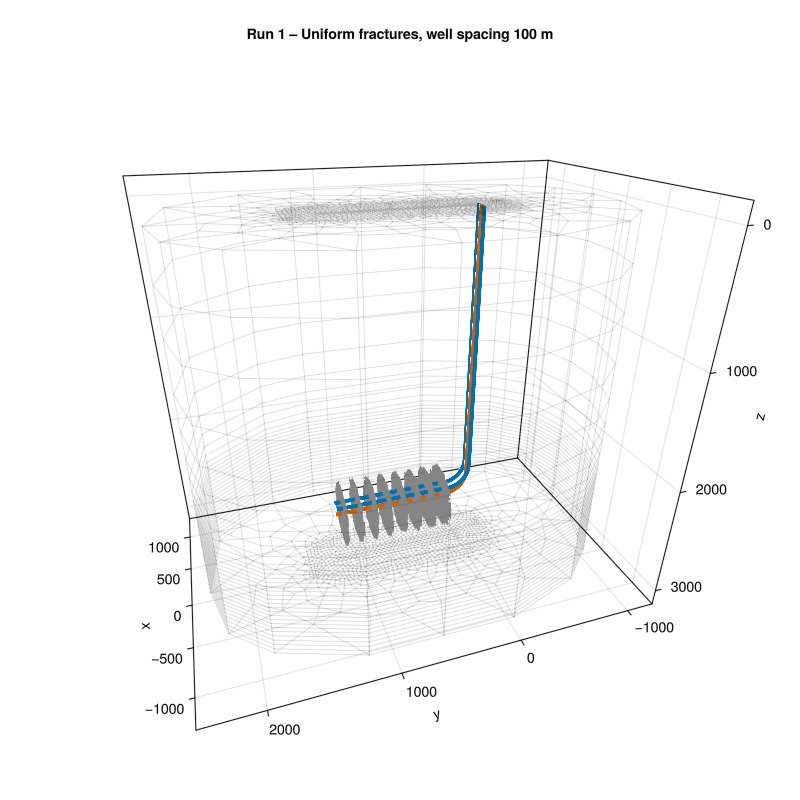

Simulate

sim, cfg = setup_egs_simulator(case)
results = simulate_reservoir(case; simulator = sim, config = cfg)

ReservoirSimResult with 113 entries:

  wells (2 present):
    :Producer
    :Injector
    Results per well:
       :lrat => Vector{Float64} of size (113,)
       :wrat => Vector{Float64} of size (113,)
       :temperature => Vector{Float64} of size (113,)
       :control => Vector{Symbol} of size (113,)
       :Aqueous_mass_rate => Vector{Float64} of size (113,)
       :bhp => Vector{Float64} of size (113,)
       :wcut => Vector{Float64} of size (113,)
       :mass_rate => Vector{Float64} of size (113,)
       :rate => Vector{Float64} of size (113,)
       :mrat => Vector{Float64} of size (113,)

  states (Vector with 113 entries, reservoir variables for each state)
    :Pressure => Vector{Float64} of size (42068,)
    :TotalMasses => Matrix{Float64} of size (1, 42068)
    :TotalThermalEnergy => Vector{Float64} of size (42068,)
    :FluidEnthalpy => Matrix{Float64} of size (1, 42068)
    :Temperature => Vector{Float64} of size (42068,)
    :PhaseMassDensities => Matrix{Float64} of size (1, 42068)
    :RockInternalEnergy => Vector{Float64} of size (42068,)
    :FluidInternalEnergy => Matrix{Float64} of size (1, 42068)

  time (report time for each state)
     Vector{Float64} of length 113

  result (extended states, reports)
     SimResult with 42 entries

  extra
     Dict{Any, Any} with keys :simulator, :config

  Completed at Apr. 30 2026 21:29 after 2 minutes, 3 seconds, 144.4 milliseconds.

Reservoir state evolution

Plot the full reservoir temperature field at all output timesteps.

msh = physical_representation(reservoir_model(case.model).data_domain)
geo = tpfv_geometry(msh)

x_range = diff(vcat(extrema(geo.cell_centroids[1, :])...))[1]
y_range = diff(vcat(extrema(geo.cell_centroids[2, :])...))[1]
z_range = diff(vcat(extrema(geo.cell_centroids[3, :])...))[1]
aspect  = (x_range, y_range, z_range) ./ max.(x_range, y_range, z_range)
plot_res_args = (
    resolution = (600, 800), aspect = aspect,
    colormap   = :seaborn_icefire_gradient, key = :Temperature,
    well_arg   = (markersize = 0.0,),
)
plot_reservoir(case.model, results.states; plot_res_args...)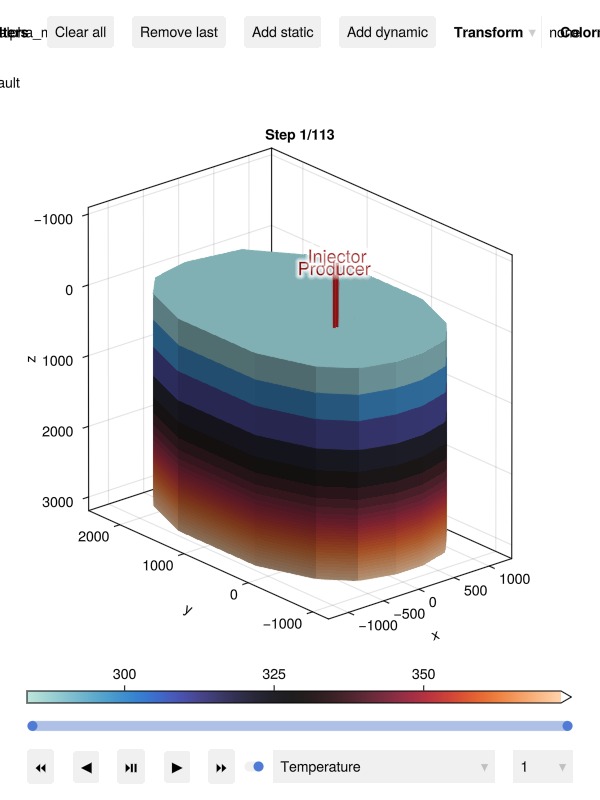

Temperature deviation from initial conditions highlights thermal depletion.

Δstates = JutulDarcy.delta_state(results.states, case.state0[:Reservoir])
plot_reservoir(case.model, Δstates; plot_res_args...)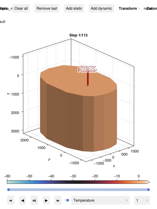

Fracture ΔT

Note that there are visual grid orientation effects in the fracture temperature distribution, contributes to accentuate differences in fracture performance. The same is also evident in the next two runs. (See note at the top of this example for details.)

plot_fracture_dt_fig(case, inj, prod, results)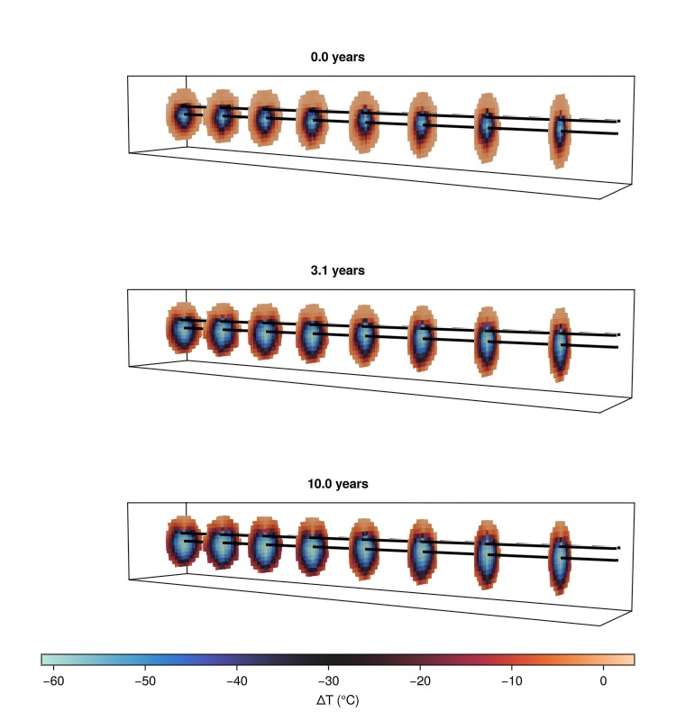

Fracture metrics

states, dt, _ = Jutul.expand_to_ministeps(results.result)
time  = cumsum(dt)  ./ si_unit(:year)
fdata = Fimbul.get_egs_fracture_data(states, case)
plot_fracture_metrics_fig(fdata, time, dt, num_years)

Run 2: Uniform fractures, 200 m well spacing

Increasing the injector–producer separation to 200 m widens the swept volume but also increases the conduction path length from rock to fracture fluid.

case2 = Fimbul.egs(inj_200, prod_200, fracture_radius, fracture_spacing;
    common_args...);
plot_egs_mesh(case2, inj_200, prod_200, "Run 2 – Uniform fractures, well spacing 200 m")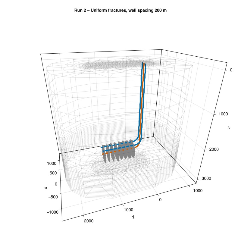

Simulate

sim2, cfg2 = setup_egs_simulator(case2)
results2 = simulate_reservoir(case2; simulator = sim2, config = cfg2)

states2, dt2, _ = Jutul.expand_to_ministeps(results2.result)
time2  = cumsum(dt2)  ./ si_unit(:year)
fdata2 = Fimbul.get_egs_fracture_data(states2, case2)

Dict{Symbol, Any} with 5 entries:
  :y                  => [250.531, 379.102, 507.673, 636.244, 764.814, 893.385,…
  :Temperature        => [358.081 358.084 … 358.134 358.175; 358.09 358.092 … 3…
  :TotalThermalEnergy => [1.30088e11 1.29206e11 … 1.29763e11 1.30215e11; 1.3009…
  :q_out              => [2.04352e7 1.92055e7 … 1.67854e7 1.67642e7; 2.15403e7 …
  :q_in               => [2.09072e7 1.94513e7 … 1.66729e7 1.66714e7; 2.24828e7 …

Well performance – Runs 1 and 2

plot_well_results([results.wells, results2.wells];
    names = ["Uniform 100 m", "Uniform 200 m"])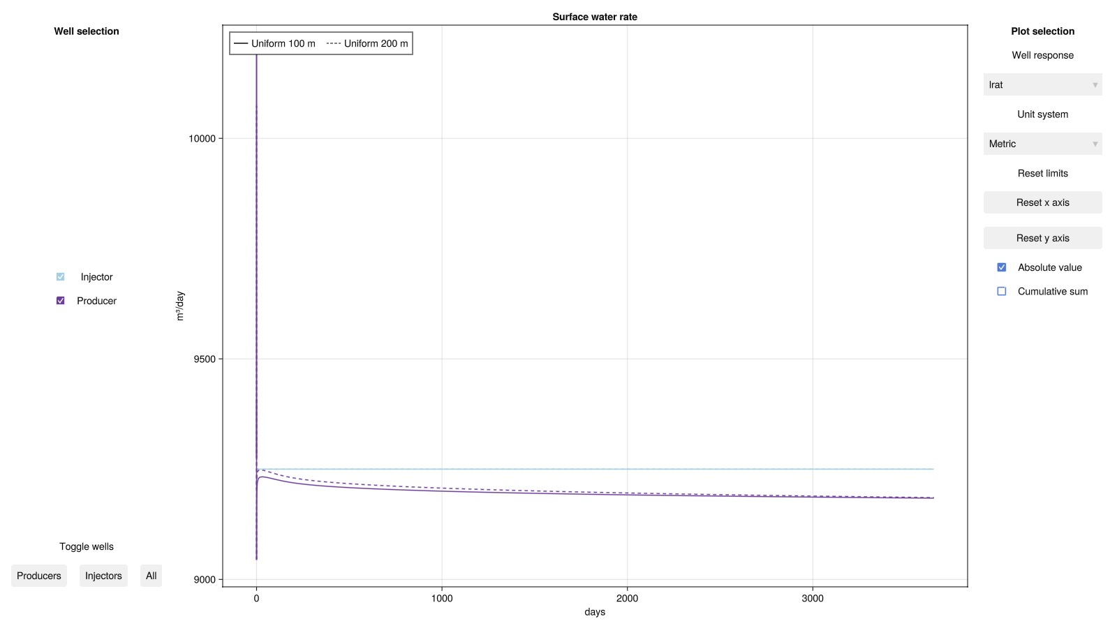

Fracture metrics – Run 2

plot_fracture_metrics_fig(fdata2, time2, dt2, num_years)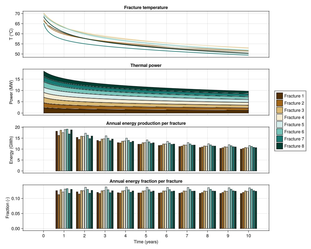

Run 3: Random fracture angles, 200 m well spacing

To understand the effect of fracture orientation, fracture angles are now sampled from N(0°, 12.5°) – a rotation around the z-axisx.

using Random
Random.seed!(20260428) # For reproducibility of random fracture anglesxs
case3 = Fimbul.egs(inj_200, prod_200, fracture_radius, fracture_spacing;
    common_args...,
    fracture_angle = (0.0, deg2rad(12.5)), # N(0°, 12.5°) rotation about z-axis
);
plot_egs_mesh(case3, inj_200, prod_200, "Run 3 – Random fractures, well spacing 200 m")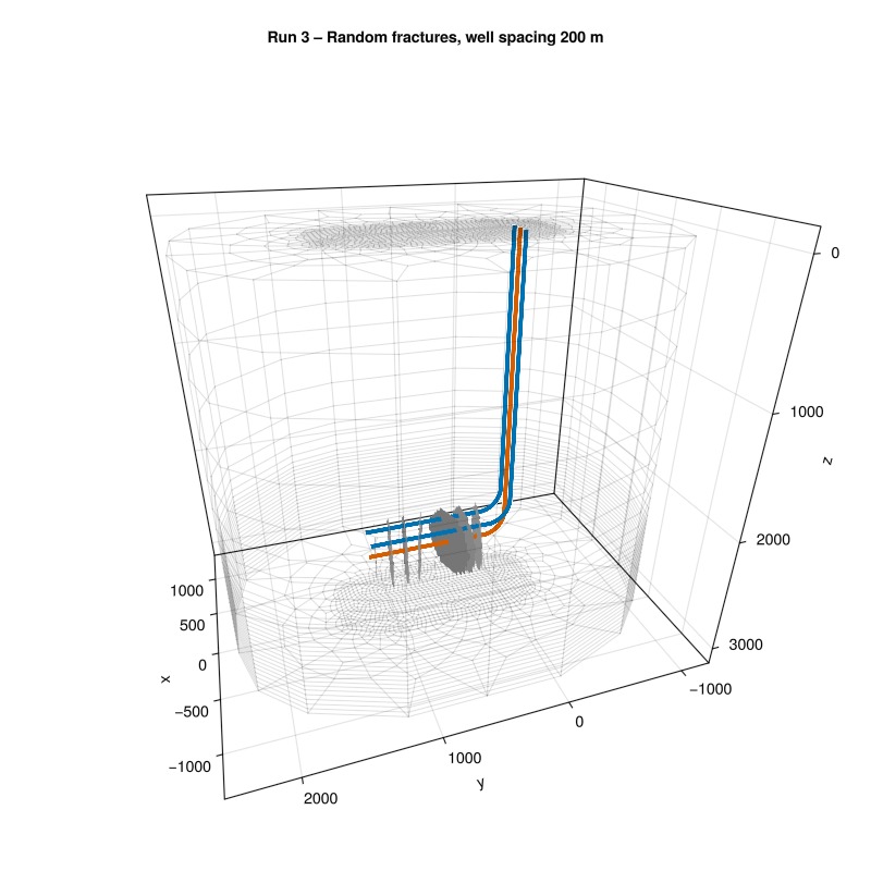

Simulate

sim3, cfg3 = setup_egs_simulator(case3)
results3 = simulate_reservoir(case3; simulator = sim3, config = cfg3)

states3, dt3, _ = Jutul.expand_to_ministeps(results3.result)
time3  = cumsum(dt3)  ./ si_unit(:year)
fdata3 = Fimbul.get_egs_fracture_data(states3, case3)

Dict{Symbol, Any} with 5 entries:
  :y                  => [250.531, 379.102, 507.673, 636.244, 764.814, 893.385,…
  :Temperature        => [358.061 357.821 … 358.133 358.149; 358.071 357.831 … …
  :TotalThermalEnergy => [1.32334e11 1.29261e11 … 1.30584e11 1.30474e11; 1.3233…
  :q_out              => [2.04857e7 1.92897e7 … 1.66706e7 1.67868e7; 2.15957e7 …
  :q_in               => [2.0925e7 1.94677e7 … 1.64997e7 1.66681e7; 2.25162e7 2…

Well performance – all three runs

plot_well_results([results.wells, results2.wells, results3.wells];
    names = ["Uniform 100 m", "Uniform 200 m", "Random 200 m"], key = :temperature)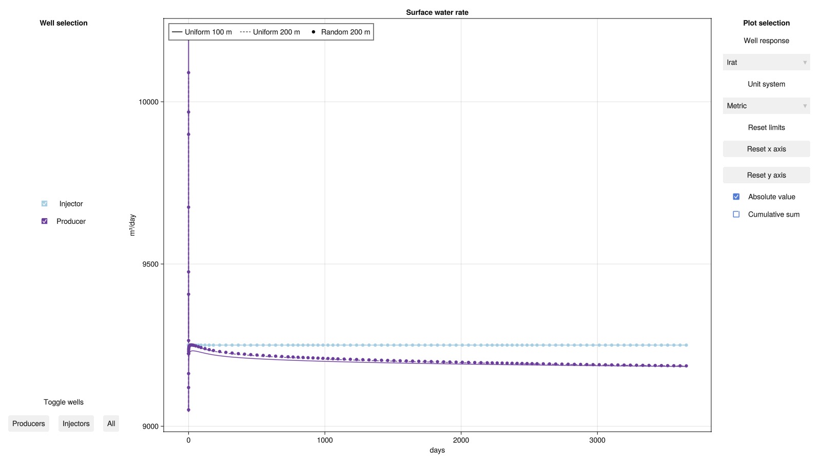

Fracture metrics – Run 3

plot_fracture_metrics_fig(fdata3, time3, dt3, num_years)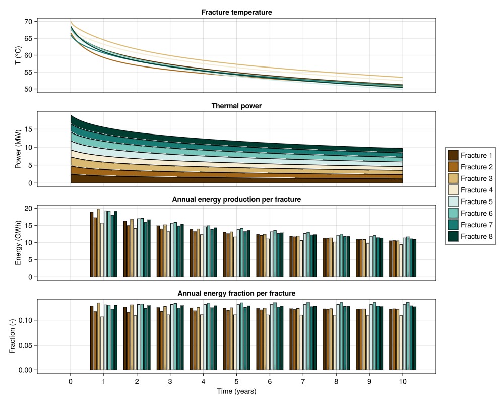

Comparison: all three runs

Compare aggregate power output, per-fracture power spread, and annual energy across the uniform 100 m, uniform 200 m and random 200 m configurations. We note that increasing well spacing from 100 m to 200 m leads to a significant drop in increase in power output, whereas the added fracture area due to angled fractures in Run 3 only provides a marginal improvement over the uniform 200 m case.

power  = fracture_power(fdata,  dt)
power2 = fracture_power(fdata2, dt2)
power3 = fracture_power(fdata3, dt3)

total_power1 = sum(power,  dims = 2)[:]
total_power2 = sum(power2, dims = 2)[:]
total_power3 = sum(power3, dims = 2)[:]

colors = Makie.wong_colors(3)

xmax_c  = round(max(maximum(time), maximum(time2), maximum(time3)))
lim_c   = ((0, xmax_c) .+ (-0.1, 0.1) .* xmax_c, nothing)
xtick_c = 0:xmax_c
fs      = findfirst(time .> 1/104)   # skip initial transient (same for all runs)

fig = Figure(size = (800, 1000))
function make_cax(title, ylabel, rno)
    Axis(fig[rno, 1]; title = title, xlabel = "Time (years)", ylabel = ylabel,
        limits = lim_c, xticks = xtick_c)
end

make_cax (generic function with 1 method)

── Total thermal power ───────────────────────────────────────────────────────

ax_c1 = make_cax("Total thermal power", "Power (MW)", 1)
lines!(ax_c1, time[fs:end],  total_power1[fs:end]  ./ 1e6;
    color = colors[1],   linewidth = 2, label = "Uniform 100 m")
lines!(ax_c1, time2[fs:end], total_power2[fs:end]  ./ 1e6;
    color = colors[2], linewidth = 2, label = "Uniform 200 m")
lines!(ax_c1, time3[fs:end], total_power3[fs:end]  ./ 1e6;
    color = colors[3],   linewidth = 2, linestyle = :dash, label = "Random 200 m")
axislegend(ax_c1; position = :rt)
hidexdecorations!(ax_c1, grid = false)

false

── Per-fracture power spread ─────────────────────────────────────────────────

ax_c2 = make_cax("Per-fracture power (shaded band = min–max)", "Power (MW)", 2)
function band_fractures!(ax, t, pwr; color = :steelblue, label = "")
    total_pwr = sum(pwr, dims = 2)[:]
    pmin = [minimum(r) for r in eachrow(pwr)]
    pmax = [maximum(r) for r in eachrow(pwr)]
    band!(ax, t, pmin ./ 1e6, pmax ./ 1e6; color = (color, 0.05), strokecolor = color, strokewidth = 1)
    lines!(ax, t, total_pwr ./ size(pwr, 2) ./ 1e6; color = color, linewidth = 3,
        label = label)
end
band_fractures!(ax_c2, time[fs:end],  power[fs:end,  :]; color = colors[1], label = "Uniform 100 m (mean)")
band_fractures!(ax_c2, time2[fs:end], power2[fs:end, :]; color = colors[2], label = "Uniform 200 m (mean)")
band_fractures!(ax_c2, time3[fs:end], power3[fs:end, :]; color = colors[3], label = "Random 200 m (mean)")
axislegend(ax_c2; position = :rt)
hidexdecorations!(ax_c2, grid = false)

false

── Annual energy ─────────────────────────────────────────────────────────────

ax_c3 = make_cax("Annual energy production", "Energy (GWh)", 3)
function annual_energy(pwr, t, dt_v)
    ix = vcat(0, [findfirst(isapprox.(t, y; atol = 1e-2)) for y in 1:num_years]) .+ 1
    [sum(pwr[ix[k]:ix[k+1]-1] .* dt_v[ix[k]:ix[k+1]-1]) / GWh for k in 1:length(ix)-1]
end
ann1 = annual_energy(total_power1, time,  dt)
ann2 = annual_energy(total_power2, time2, dt2)
ann3 = annual_energy(total_power3, time3, dt3)
years = 1:num_years
args = (width = 0.25, strokecolor=:black, strokewidth=1)
barplot!(ax_c3, years .- 0.28, ann1; args..., color = colors[1], label = "Uniform 100 m")
barplot!(ax_c3, years,         ann2; args..., color = colors[2], label = "Uniform 200 m")
barplot!(ax_c3, years .+ 0.28, ann3; args..., color = colors[3], label = "Random 200 m")
axislegend(ax_c3; position = :rt)

fig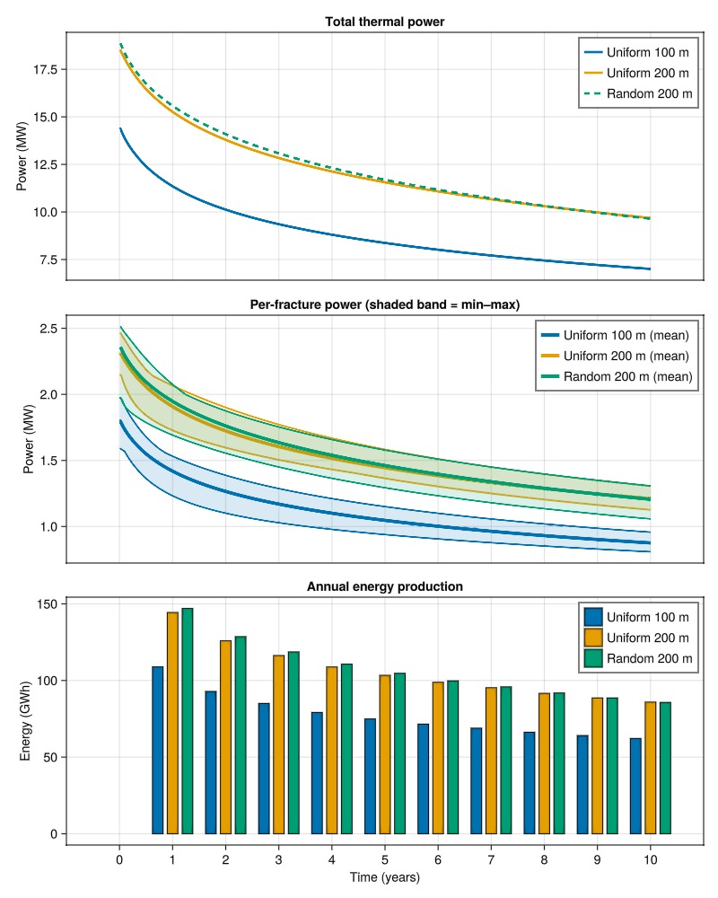

Example on GitHub

If you would like to run this example yourself, it can be downloaded from the Fimbul.jl GitHub repository as a script.

This example took 428.322420648 seconds to complete.

---

This page was generated using Literate.jl.