
Design optimization of a multi-well coaxial BHE system
Production WorkflowThis example demonstrates how simulations can be used to design a system of deep coaxial borehole heat exchangers (BHEs). We consider four coaxial BHEs placed in a circular pattern with radius r_surf at the surface. Down to a kickoff depth of 250 m, the wells are vertical. Below this, they deviate outwards at an angle θ from the vertical, so that the wells lie on the surface of a cone. The drilled length L of each well (measured along the well) is at most 2000 m. We seek the tilt angle and the well length that minimize the drilling costs, under the constraint that the average thermal power of the system over N years is at least Q.
The design variables affect the system in several ways:
With vertical wells close to each other, the wells compete for the heat in the same rock volume, and the thermal interference reduces the power. Tilting the wells increases the distance between them.
Tilted wells reach shallower depths, where the rock is colder, which reduces the power. Tilted wells are also more expensive to drill.
Longer wells give more power, but are more expensive.
See the coaxial BHE demo for more details on the coaxial BHE setup, and for the calibration of the layered thermal conductivity used here.
Add required modules to namespace
using Jutul, JutulDarcy, Fimbul
using HYPRE
using GLMakie
Useful SI units
meter, hour, watt, Kelvin, joule, kilogram, year, atm = si_units(
    :meter, :hour, :watt, :Kelvin, :joule, :kilogram, :year, :atm
);
Design parameters
r_surf = 25.0meter
kickoff = 250.0meter
L_max = 2000.0meter
N_years = 20
Q_min = 0.8e6watt;
Geology and operational parameters
The geology consists of three layers, where the middle layer has a distinctly lower thermal conductivity than the other two. These are the conductivities obtained by calibrating a digital twin to downhole temperature measurements in the coaxial BHE demo. Each well is operated with the same rate and injection temperature as in the coaxial BHE demo, with injection into the outer annulus and production from the inner pipe.
λ_unit = watt / (meter * Kelvin)
depths_layers = [0.0, 800.0, 1700.0, 3000.0]
λ_layers = [3.0, 1.5, 3.5] * λ_unit
num_layers = length(λ_layers)
rate = 25meter^3 / hour
temperature_inj = convert_to_si(10.0, :Celsius);
Drilling costs
The cost of drilling a well increases more than linearly with its measured depth (drilled length). We use the correlation of [] for the drilling and completion cost of geothermal wells, C(L) = 1.72e-7 L² + 2.3e-3 L - 0.62 million USD, with L the measured depth in meters, which we for simplicity use in million €. Since a coaxial BHE requires a smaller borehole than a geothermal production well, we scale the cost by a factor f_slim. Directional drilling is more expensive than vertical drilling, due to, e.g., directional drilling services and increased torque and drag. We account for this with a surcharge that increases with the tilt angle and the deviated fraction of the well.
f_slim = 0.6 # Cost factor for the smaller borehole of a coaxial BHE
α_dev = 0.3 # Maximum surcharge for directional drilling
lukawski_cost(L) = 1.0e6 * (1.72e-7 * L^2 + 2.3e-3 * L - 0.62)
function drilling_cost(θ, L; num_wells = 4)
    surcharge = 1 + α_dev * sin(θ) * (L - kickoff) / L
    return num_wells * f_slim * lukawski_cost(L) * surcharge
end;
Well trajectories
The trajectories of the four wells are given by the surface location, the kickoff point and the end point of each well. The pattern is rotated by 45°, so that the wells lie on the diagonals of the quarter domains used for the simulations below.
function pattern_trajectories(θ, L = L_max)
    return map((π / 4, 3π / 4, 5π / 4, 7π / 4)) do φ
        r = [r_surf, r_surf, r_surf + (L - kickoff) * sin(θ)]
        z = [0.0, kickoff, kickoff + (L - kickoff) * cos(θ)]
        hcat(r .* cos(φ), r .* sin(φ), z)
    end
end

function plot_trajectory!(ax, trajectory; color = :black, linewidth = 4, kwarg...)
    return lines!(
        ax, trajectory[:, 1], trajectory[:, 2], trajectory[:, 3];
        color = color, linewidth = linewidth, kwarg...
    )
end;
Simulation model
Due to the symmetry of the pattern, we only need to simulate a quarter of the domain, containing one of the wells: The vertical planes through the center of the pattern (x = 0 and y = 0) are symmetry planes without flow of mass or heat. The thermal interference between the wells is thus accounted for, since each well cannot extract heat from beyond the symmetry planes.
We use a tensor mesh that is adapted to each design: The cells are 25 m horizontally from the symmetry planes to 100 m beyond the end of the well, and 100 m vertically down to 100 m below the bottom of the well. Outside these regions, the cell sizes increase geometrically towards the outer boundaries of the domain, which is 2000 m wide and 3000 m deep.
function graded_cells(L_fine, h, L_total; growth = 1.5)
    d = fill(h, ceil(Int, L_fine / h))
    while sum(d) < L_total
        push!(d, min(d[end] * growth, L_total - sum(d)))
    end
    return d
end;
The wells are close to each other in the vertical section above the kickoff depth. To limit the thermal interference there, the upper section of each well is thermally insulated, using a grout with a very low thermal conductivity. This is also a reasonable choice from an operational point of view, since the shallow rock is cold and contributes little to the heat extraction, and the insulation reduces the heat loss from the produced fluid on its way up. Below the kickoff depth, the default grout is used.
λ_grout = 2.3λ_unit
λ_grout_insulated = 0.01λ_unit

function design_case(θ, L; margin = 100.0)
    # The well in the quarter domain x, y > 0
    trajectory = first(pattern_trajectories(θ, L))
    x_end, z_end = trajectory[end, 1], trajectory[end, 3]
    dxy = graded_cells(x_end + margin, 25.0, 2000.0)
    dz = graded_cells(z_end + margin, 100.0, 3000.0)
    mesh = UnstructuredMesh(
        CartesianMesh(
            (length(dxy), length(dxy), length(dz)), (dxy, dxy, dz)
        )
    )
    geo = tpfv_geometry(mesh)
    zc = geo.cell_centroids[3, :]
    layer = [clamp(searchsortedlast(depths_layers, z), 1, num_layers) for z in zc]
    domain = Fimbul.layered_reservoir_domain(
        mesh, layer, (
            permeability = 1.0e-3 * si_unit(:darcy),
            porosity = 0.01,
            rock_thermal_conductivity = λ_layers,
            rock_heat_capacity = 900 * joule / (kilogram * Kelvin),
            rock_density = 2600 * kilogram / meter^3,
        )
    )
    cells, extra = Jutul.find_enclosing_cells(mesh, trajectory, extra_out = true)
    # Insulating grout in the vertical section above the kickoff depth, based
    # on the depth of the trajectory in each well cell
    z_traj = [c[3] for c in extra[:centroids]]
    grout = ifelse.(z_traj .< kickoff, λ_grout_insulated, λ_grout)
    # The closed-loop well is a single merged well, :BHE, controlled as
    # :BHE_inner and :BHE_outer (see `closed_loop_well_names`)
    well = setup_closed_loop_well(
        domain, cells; name = :BHE,
        closed_loop_type = :coaxial,
        dir = Vector.(extra[:direction] .* extra[:lengths]),
        fill_thermal_conductivity = grout
    )
    model = setup_reservoir_model(
        domain, :geothermal; wells = [well],
        energy_formulation = :total, can_shut_wells = false
    )
    # Fixed pressure and temperature at the top, bottom and outer sides, with
    # the same surface conditions and gradients as in the coaxial BHE case
    ρ = reservoir_model(model).system.rho_ref[1]
    p(z) = 10atm + ρ * gravity_constant * z
    T(z) = convert_to_si(10.0, :Celsius) + 0.03z
    X, Z = sum(dxy), sum(dz)
    bc_cells, bc_z = Int[], Float64[]
    for (i, c) in enumerate(geo.boundary_neighbors)
        x, y, z = geo.boundary_centroids[:, i]
        if isapprox(z, 0.0, atol = 1.0e-6) || isapprox(z, Z) || isapprox(x, X) || isapprox(y, X)
            push!(bc_cells, c)
            push!(bc_z, z)
        end
    end
    bc = flow_boundary_condition(bc_cells, domain, p.(bc_z), T.(bc_z))
    state0 = setup_reservoir_state(model, Pressure = p.(zc), Temperature = T.(zc))
    zw = model.models[:BHE].data_domain[:cell_centroids][3, :]
    state0[:BHE][:Pressure] .= p.(zw)
    state0[:BHE][:Temperature] .= T.(zw)
    # Injection into the outer annulus, production from the inner pipe
    control = Dict(
        :BHE_inner => ProducerControl(BottomHolePressureTarget(5atm)),
        :BHE_outer => InjectorControl(
            TotalRateTarget(rate), [1.0],
            density = ρ, temperature = temperature_inj
        )
    )
    forces = setup_reservoir_forces(model, control = control, bc = bc)
    dt, forces = make_schedule(
        [forces], [(1, 1), (1, 1)];
        num_years = N_years, report_interval = year / 4
    )
    return JutulCase(
        model, dt, forces; state0 = state0,
        input_data = Dict(:trajectory => trajectory)
    )
end

function run_case(case)
    sim, cfg = setup_reservoir_simulator(
        case;
        info_level = -1,
        initial_dt = 120.0,
        presolve_wells = true,
        relaxation = true
    )
    for model in (:Reservoir, :BHE)
        sel = VariableChangeTimestepSelector(
            :Temperature, 5.0;
            relative = false, model = model
        )
        push!(cfg[:timestep_selectors], sel)
    end
    return simulate_reservoir(case; simulator = sim, config = cfg)
end;
Thermal power
The thermal power of the system is the power of the simulated well multiplied by four, computed from the mass rate and the temperature difference between production and injection. We compute the average power over the first N years of operation.
function system_power(results; c_p = 4184.0joule / (kilogram * Kelvin))
    w = results.wells[:BHE_inner]
    return 4 .* abs.(w[:mass_rate]) .* c_p .* (w[:temperature] .- temperature_inj)
end

function average_power(results, N = N_years)
    t = results.time
    dt = diff([0.0; t])
    active = t .<= N * year + 1.0
    P = system_power(results)
    return sum(P[active] .* dt[active]) / sum(dt[active])
end;
Evaluate designs
Since the mesh and well geometry change with the design, we cannot use the adjoint method to compute gradients with respect to the design variables. Instead, we evaluate the designs on a grid of tilt angles and well lengths, which is affordable since the problem only has two design variables.
θ_values = deg2rad.(0.0:10.0:60.0)
L_values = collect(1000.0:250.0:L_max)
function simulate_design(θ, L)
    println("Simulating design θ = $(round(rad2deg(θ), digits = 2))°, L = $(round(L, digits = 1)) m, drilling cost $(round(drilling_cost(θ, L) / 1.0e6, digits = 2)) M€")
    return run_case(design_case(θ, L))
end

design_results = [simulate_design(θ, L) for θ in θ_values, L in L_values]
P_avg = average_power.(design_results)
costs = [drilling_cost(θ, L) for θ in θ_values, L in L_values];
Simulating design θ = 0.0°, L = 1000.0 m, drilling cost 4.44 M€
Simulating design θ = 10.0°, L = 1000.0 m, drilling cost 4.62 M€
Simulating design θ = 20.0°, L = 1000.0 m, drilling cost 4.79 M€
Simulating design θ = 30.0°, L = 1000.0 m, drilling cost 4.94 M€
Simulating design θ = 40.0°, L = 1000.0 m, drilling cost 5.09 M€
Simulating design θ = 50.0°, L = 1000.0 m, drilling cost 5.21 M€
Simulating design θ = 60.0°, L = 1000.0 m, drilling cost 5.31 M€
Simulating design θ = 0.0°, L = 1250.0 m, drilling cost 6.06 M€
Simulating design θ = 10.0°, L = 1250.0 m, drilling cost 6.31 M€
Simulating design θ = 20.0°, L = 1250.0 m, drilling cost 6.55 M€
Simulating design θ = 30.0°, L = 1250.0 m, drilling cost 6.78 M€
Simulating design θ = 40.0°, L = 1250.0 m, drilling cost 6.99 M€
Simulating design θ = 50.0°, L = 1250.0 m, drilling cost 7.17 M€
Simulating design θ = 60.0°, L = 1250.0 m, drilling cost 7.32 M€
Simulating design θ = 0.0°, L = 1500.0 m, drilling cost 7.72 M€
Simulating design θ = 10.0°, L = 1500.0 m, drilling cost 8.06 M€
Simulating design θ = 20.0°, L = 1500.0 m, drilling cost 8.38 M€
Simulating design θ = 30.0°, L = 1500.0 m, drilling cost 8.69 M€
Simulating design θ = 40.0°, L = 1500.0 m, drilling cost 8.96 M€
Simulating design θ = 50.0°, L = 1500.0 m, drilling cost 9.2 M€
Simulating design θ = 60.0°, L = 1500.0 m, drilling cost 9.39 M€
Simulating design θ = 0.0°, L = 1750.0 m, drilling cost 9.44 M€
Simulating design θ = 10.0°, L = 1750.0 m, drilling cost 9.86 M€
Simulating design θ = 20.0°, L = 1750.0 m, drilling cost 10.27 M€
Simulating design θ = 30.0°, L = 1750.0 m, drilling cost 10.65 M€
Simulating design θ = 40.0°, L = 1750.0 m, drilling cost 11.0 M€
Simulating design θ = 50.0°, L = 1750.0 m, drilling cost 11.29 M€
Simulating design θ = 60.0°, L = 1750.0 m, drilling cost 11.54 M€
Simulating design θ = 0.0°, L = 2000.0 m, drilling cost 11.2 M€
Simulating design θ = 10.0°, L = 2000.0 m, drilling cost 11.71 M€
Simulating design θ = 20.0°, L = 2000.0 m, drilling cost 12.21 M€
Simulating design θ = 30.0°, L = 2000.0 m, drilling cost 12.67 M€
Simulating design θ = 40.0°, L = 2000.0 m, drilling cost 13.09 M€
Simulating design θ = 50.0°, L = 2000.0 m, drilling cost 13.46 M€
Simulating design θ = 60.0°, L = 2000.0 m, drilling cost 13.75 M€Tested configurations
We plot the trajectories of the four wells for all tested tilt angles with the maximum well length. The shorter wells follow the same trajectories, but end earlier.
fig = Figure(size = (900, 700))
ax = Axis3(
    fig[1, 1]; zreversed = true, perspectiveness = 0.75, aspect = :data,
    title = "Tested well configurations (L = $(round(Int, L_max)) m)",
    xlabel = "x (m)", ylabel = "y (m)", zlabel = "Depth (m)"
)
cmap_θ = cgrad(:viridis, length(θ_values), categorical = true)
for (i, θ) in enumerate(θ_values)
    for trajectory in pattern_trajectories(θ)
        plot_trajectory!(ax, trajectory; color = cmap_θ[i], linewidth = 3)
    end
end
Colorbar(
    fig[1, 2]; colormap = cmap_θ, limits = rad2deg.(extrema(θ_values)),
    label = "Tilt angle θ (°)"
)
fig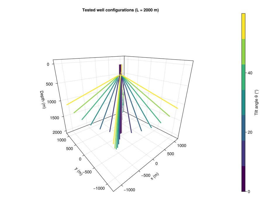
Power over time
The power drops quickly during the first months of operation, as the rock close to the wells is cooled. For vertical wells, the drop continues for longer, as the cooled regions around the wells start to overlap. We show the results for the maximum well length.
fig = Figure(size = (800, 500))
ax = Axis(
    fig[1, 1]; title = "Thermal power of the four-well system (L = $(round(Int, L_max)) m)",
    xlabel = "Time (years)", ylabel = "Power (MW)"
)
for (i, θ) in enumerate(θ_values)
    r = design_results[i, end]
    lines!(
        ax, r.time ./ year, system_power(r) ./ 1.0e6; color = cmap_θ[i],
        label = "$(round(Int, rad2deg(θ)))°"
    )
end
Legend(fig[1, 2], ax, "Tilt angle")
fig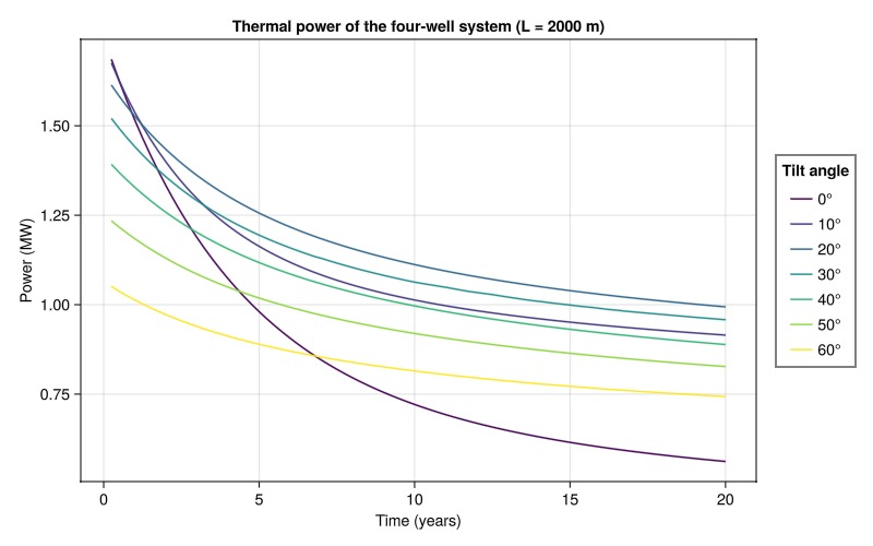
Optimal design
We interpolate the average power bilinearly between the evaluated designs, and find the design with the lowest drilling cost that satisfies the power constraint on a fine grid of tilt angles and well lengths. For a given well length, the cheapest feasible design is the smallest tilt angle that gives sufficient power, since the cost increases with the tilt angle. The optimal design is then verified with a simulation. If the interpolation was too optimistic, the wells are lengthened slightly until the constraint is satisfied. Note that the power is not exactly a smooth function of the design variables, since the mesh and the cells the well passes through change with the design.
function interpolate_power(P, θ, L)
    i = clamp(searchsortedlast(θ_values, θ), 1, length(θ_values) - 1)
    j = clamp(searchsortedlast(L_values, L), 1, length(L_values) - 1)
    s = (θ - θ_values[i]) / (θ_values[i + 1] - θ_values[i])
    t = (L - L_values[j]) / (L_values[j + 1] - L_values[j])
    return (1 - s) * (1 - t) * P[i, j] + s * (1 - t) * P[i + 1, j] +
        (1 - s) * t * P[i, j + 1] + s * t * P[i + 1, j + 1]
end

θ_fine = deg2rad.(0.0:0.25:60.0)
L_fine = collect(1000.0:5.0:L_max)
function optimal_design(P, Q)
    best = (Inf, NaN, NaN)
    for θ in θ_fine, L in L_fine
        interpolate_power(P, θ, L) >= Q || continue
        C = drilling_cost(θ, L)
        C < best[1] && (best = (C, θ, L))
    end
    return best
end

_, θ_opt, L_opt = optimal_design(P_avg, Q_min)
isnan(θ_opt) && error("No design satisfies the power constraint")
P_opt = 0.0
for it in 1:5
    global P_opt = average_power(simulate_design(θ_opt, L_opt))
    println("Verification $it: θ = $(round(rad2deg(θ_opt), digits = 2))°, L = $(round(L_opt, digits = 1)) m, average power $(round(P_opt / 1.0e6, digits = 4)) MW")
    P_opt >= Q_min && break
    global L_opt = min(L_opt + 25.0, L_max)
end
C_opt = drilling_cost(θ_opt, L_opt)
println("Optimal design: θ = $(round(rad2deg(θ_opt), digits = 1))°, L = $(round(L_opt, digits = 1)) m, average power $(round(P_opt / 1.0e6, digits = 3)) MW, drilling cost $(round(C_opt / 1.0e6, digits = 2)) M€")
Simulating design θ = 20.0°, L = 1505.0 m, drilling cost 8.42 M€
Verification 1: θ = 20.0°, L = 1505.0 m, average power 0.7995 MW
Simulating design θ = 20.0°, L = 1530.0 m, drilling cost 8.6 M€
Verification 2: θ = 20.0°, L = 1530.0 m, average power 0.8191 MW
Optimal design: θ = 20.0°, L = 1530.0 m, average power 0.819 MW, drilling cost 8.6 M€Design space
The left plot shows the average power as a function of the tilt angle and the well length, with the boundary of the feasible region (white line, where the power is equal to the requirement). The right plot shows the drilling cost. The optimal design lies on the boundary of the feasible region: It is the shortest well that can satisfy the requirement, with the tilt angle that gives (close to) the most power for this length.
θ_deg = rad2deg.(θ_values)
fig = Figure(size = (1100, 450))
ax_p = Axis(
    fig[1, 1]; title = "Average power over $(N_years) years",
    xlabel = "Tilt angle θ (°)", ylabel = "Well length L (m)"
)
hm = contourf!(ax_p, θ_deg, L_values, P_avg ./ 1.0e6; levels = 15, colormap = :viridis)
contour!(
    ax_p, θ_deg, L_values, P_avg ./ 1.0e6; levels = [Q_min / 1.0e6],
    color = :white, linewidth = 3
)
scatter!(
    ax_p, vec([t for t in θ_deg, L in L_values]), vec([L for t in θ_deg, L in L_values]);
    color = :black, markersize = 5
)
scatter!(ax_p, [rad2deg(θ_opt)], [L_opt]; marker = :star5, markersize = 22, color = :orange)
Colorbar(fig[1, 2], hm; label = "Power (MW)")
ax_c = Axis(
    fig[1, 3]; title = "Drilling cost",
    xlabel = "Tilt angle θ (°)", ylabel = "Well length L (m)"
)
hc = contourf!(ax_c, θ_deg, L_values, costs ./ 1.0e6; levels = 15, colormap = :magma)
contour!(
    ax_c, θ_deg, L_values, P_avg ./ 1.0e6; levels = [Q_min / 1.0e6],
    color = :white, linewidth = 3
)
scatter!(ax_c, [rad2deg(θ_opt)], [L_opt]; marker = :star5, markersize = 22, color = :orange)
Colorbar(fig[1, 4], hc; label = "Cost (M€)")
fig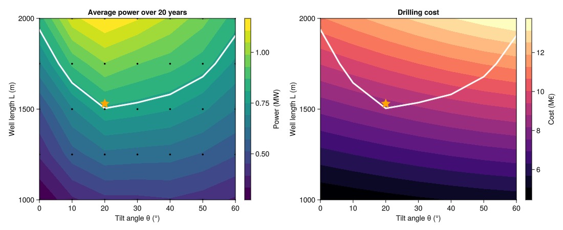
Optimal configuration
The four wells of the optimal design.
fig = Figure(size = (700, 650))
ax = Axis3(
    fig[1, 1]; zreversed = true, perspectiveness = 0.75, aspect = :data,
    title = "Optimal design: θ = $(round(rad2deg(θ_opt), digits = 1))°, L = $(round(Int, L_opt)) m",
    xlabel = "x (m)", ylabel = "y (m)", zlabel = "Depth (m)"
)
for trajectory in pattern_trajectories(θ_opt, L_opt)
    plot_trajectory!(ax, trajectory; color = :orange, linewidth = 4)
end
fig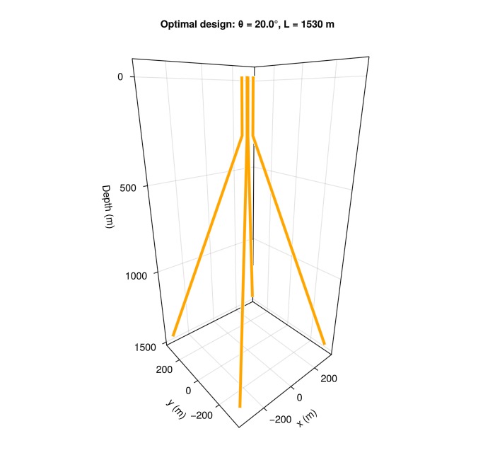
Cost of the power requirement
The optimal design depends on the requirements. To illustrate this, we compute the minimum drilling cost as a function of the required average power, for operation periods of 5 and 20 years, using the interpolated power, which requires no additional simulations. Over a shorter period, the cooled regions around the wells have less time to grow and interfere, so that a higher average power can be achieved for the same cost.
fig = Figure(size = (700, 450))
ax = Axis(
    fig[1, 1]; title = "Minimum drilling cost",
    xlabel = "Required average power (MW)", ylabel = "Cost (M€)"
)
for (N, color) in ((5, :steelblue), (N_years, :darkorange))
    P_N = [average_power(r, N) for r in design_results]
    Q_range = range(minimum(P_N), 0.99maximum(P_N), length = 40)
    C_min = [first(optimal_design(P_N, Q)) for Q in Q_range]
    lines!(
        ax, Q_range ./ 1.0e6, C_min ./ 1.0e6; color = color, linewidth = 3,
        label = "$N years"
    )
end
scatter!(
    ax, [P_opt / 1.0e6], [C_opt / 1.0e6]; marker = :star5,
    markersize = 20, color = :orange, label = "Optimal design"
)
axislegend(ax; position = :lt)
fig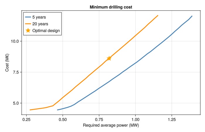
Download this example
Download the Julia script or the Jupyter notebook.
This example took 349.085517362 seconds to complete.This page was generated using Literate.jl.