1D high-temperature geothermal benchmark
ValidationThis example reproduces the 1D high-temperature geothermal benchmark cases from [5] using the pressure-enthalpy formulation in Fimbul, and validates the results against HYDROTHERM [6] reference solutions.
using Jutul, JutulDarcy, Fimbul, GLMakie

to_celsius(T) = convert_from_si.(T, :Celsius)
to_megapascal(p) = convert_from_si.(p, "megapascal")
to_kj_per_kg(h) = h ./ 1e3

const SINGLE_PHASE_CASES = (:a, :b, :c)
const TWO_PHASE_CASES = (:d, :e)
const CASE_COLORS = Dict(
    :a => :blue,
    :b => :red,
    :c => :lightgreen,
    :d => :cyan,
    :e => :magenta,
)
const PROFILE_SPECS = (
    (name = :Pressure, label = "Pressure [MPa]", transform = to_megapascal,
        hydrotherm_column = "pressure_mpa"),
    (name = :Temperature, label = "Temperature [°C]", transform = to_celsius,
        hydrotherm_column = "temperature_c"),
    (name = :Saturations, label = "Liquid saturation [-]", transform = x -> vec(x[1,:]),
        hydrotherm_column = "liquid_saturation"),
)

nx = 200
cell_size = 10.0;
Utilities
function simulate_benchmark_case(case_symbol; vertical = false, nx = 100, cell_size = 10.0)

    case = benchmark_ht_1d(
        benchmark_case = case_symbol,
        nx = nx,
        cell_size = cell_size,
        vertical = vertical,
    )
    case = Fimbul.replace_case_timesteps(
        case,
        Fimbul.load_hydrotherm_1d_timesteps(case_symbol, vertical);
        check_sum = true,
    )
    simulator, config = setup_reservoir_simulator(
        case;
        tol_cnv = 1e-3,
        tol_mb = 1e-7,
        max_timestep = Inf,
        timesteps = :none,
        relaxation = true,
    )
    results = simulate_reservoir(case; simulator = simulator, config = config)
    return (case = case, results = results)
end

function simulate_case_family(case_symbols; nx = 100, cell_size = 10.0)

    outputs = Dict{Tuple{Symbol, Bool}, Any}()
    for case_symbol in case_symbols
        for vertical in Fimbul.available_vertical_modes_ht_1d(case_symbol)
            @info "Simulating case $(case_symbol) with vertical = $(vertical)"
            outputs[(case_symbol, vertical)] = simulate_benchmark_case(
                case_symbol;
                vertical = vertical,
                nx = nx,
                cell_size = cell_size,
            )
        end
    end
    return outputs
end

function reservoir_coordinate(out)
    domain = out.case.model.models[:Reservoir].data_domain
    centroids = tpfv_geometry(physical_representation(domain)).cell_centroids
    if out.case.input_data[:vertical]
        return vec(centroids[3, :])
    else
        return vec(centroids[1, :])
    end
end

function ordered_values(values, vertical)
    values = vec(values)
    return vertical ? reverse(values) : values
end

function plot_property_maps(tables)
    specs = (
        (
            variable = :temperature,
            label = "Temperature [°C]",
        ),
        (
            variable = :density_mix,
            label = "Density [kg/m³]",
        ),
        (
            variable = :saturation_vapor_ph,
            label = "Vapor saturation [-]",
        ),
    )

    fig = Figure(size = (1200, 500))
    for (i, spec) in enumerate(specs)
        yaxisposition = ifelse(i < length(specs), :left, :right)
        ax = Axis(fig[2, i];
            xticksmirrored = true, yticksmirrored = true,
            yaxisposition = yaxisposition, aspect = AxisAspect(1))
        handles = Fimbul.plot_phase_diagram_contours!(
            ax,
            tables;
            variable = spec.variable,
            pressure_limits = (1e5, 52.5e6),
            enthalpy_limits = (500e3, 3500e3),
            n_pressure = 500,
            n_enthalpy = 500,
            levels = 18,
            lines = true,
            contourf_kwargs = (; colormap = :seaborn_icefire_gradient),
        )
        Colorbar(fig[1, i], handles.filled, vertical = false, flipaxis = true, width = ax.width,
            label = spec.label, labelsize = 20)
        if i > 1
            hideydecorations!(ax, ticks = false)
        end
    end
    is_ax = [f isa Axis for f in fig.content]
    linkaxes!(fig.content[is_ax]...)
    return fig
end

function plot_case_profiles(case_symbol, results)
    vertical_modes = Fimbul.available_vertical_modes_ht_1d(case_symbol)
    fig_height = 400 * length(vertical_modes)
    fig = Figure(size = (800 + 400*(case_symbol ∈ TWO_PHASE_CASES), fig_height))

    for (k, vertical) in enumerate(vertical_modes)
        out = results[(case_symbol, vertical)]
        x = reservoir_coordinate(out)
        state = out.results.states[end]

        row = 2*(k-1)
        vertical_label = vertical ? "vertical" : "horizontal"
        for (col, spec) in enumerate(PROFILE_SPECS)
            if spec.name == :Saturations && case_symbol ∉ TWO_PHASE_CASES
                continue
            end
            values = spec.transform(state[spec.name])
            hydrotherm = Fimbul.load_hydrotherm_1d_property(case_symbol, vertical, spec.hydrotherm_column)
            if vertical
                ax = Axis(
                    fig[row+1, col];
                    xlabel = spec.label,
                    ylabel = "Depth [m]",
                    yreversed = true,
                )
                if hydrotherm !== nothing
                    lines!(ax, hydrotherm.values, hydrotherm.coordinate_m .- cell_size/2;
                        linewidth = 8, linestyle = :dash, color = :black, label = "HYDROTHERM")
                end
                lines!(ax, values, x, color = CASE_COLORS[case_symbol], linewidth = 3, label = "Fimbul")
            else
                ax = Axis(
                    fig[row+1, col];
                    xlabel = "Distance [m]",
                    ylabel = spec.label,
                )
                y = ordered_values(values, vertical)
                if hydrotherm !== nothing
                    lines!(ax, hydrotherm.coordinate_m .- cell_size/2, hydrotherm.values;
                        linewidth = 8, linestyle = :dash, color = :black, label = "HYDROTHERM")
                end
                lines!(ax, x, y, color = CASE_COLORS[case_symbol], linewidth = 3, label = "Fimbul")
                if col == 1
                    axislegend(ax; position = :rt)
                end
            end
        end
        fig[row, :] = Label(fig, "Case $(case_symbol) ($(vertical_label))"; fontsize = 20)
    end
    return fig
end;
Simulate all cases
all_results = simulate_case_family(
    (SINGLE_PHASE_CASES..., TWO_PHASE_CASES...);
    nx = nx, cell_size = cell_size);
[ Info: Simulating case a with vertical = false
Jutul: Simulating 250 years, 3.993 weeks as 109 report steps
╭────────────────┬───────────┬───────────────┬──────────╮
│ Iteration type │ Avg/step │ Avg/ministep │ Total │
│ │ 109 steps │ 111 ministeps │ (wasted) │
├────────────────┼───────────┼───────────────┼──────────┤
│ Newton │ 2.01835 │ 1.98198 │ 220 (0) │
│ Linearization │ 3.0367 │ 2.98198 │ 331 (0) │
│ Linear solver │ 2.01835 │ 1.98198 │ 220 (0) │
│ Precond apply │ 4.0367 │ 3.96396 │ 440 (0) │
╰────────────────┴───────────┴───────────────┴──────────╯
╭───────────────┬─────────┬────────────┬────────╮
│ Timing type │ Each │ Relative │ Total │
│ │ ms │ Percentage │ s │
├───────────────┼─────────┼────────────┼────────┤
│ Properties │ 0.1114 │ 0.51 % │ 0.0245 │
│ Equations │ 2.8905 │ 19.91 % │ 0.9568 │
│ Assembly │ 0.8047 │ 5.54 % │ 0.2664 │
│ Linear solve │ 0.6507 │ 2.98 % │ 0.1432 │
│ Linear setup │ 0.9335 │ 4.27 % │ 0.2054 │
│ Precond apply │ 0.0392 │ 0.36 % │ 0.0172 │
│ Update │ 1.9426 │ 8.89 % │ 0.4274 │
│ Convergence │ 3.0205 │ 20.80 % │ 0.9998 │
│ Input/Output │ 0.5421 │ 1.25 % │ 0.0602 │
│ Other │ 7.7503 │ 35.48 % │ 1.7051 │
├───────────────┼─────────┼────────────┼────────┤
│ Total │ 21.8445 │ 100.00 % │ 4.8058 │
╰───────────────┴─────────┴────────────┴────────╯
[ Info: Simulating case a with vertical = true
Jutul: Simulating 749 years, 35.04 weeks as 85 report steps
╭────────────────┬──────────┬──────────────┬──────────╮
│ Iteration type │ Avg/step │ Avg/ministep │ Total │
│ │ 85 steps │ 87 ministeps │ (wasted) │
├────────────────┼──────────┼──────────────┼──────────┤
│ Newton │ 2.01176 │ 1.96552 │ 171 (0) │
│ Linearization │ 3.03529 │ 2.96552 │ 258 (0) │
│ Linear solver │ 2.01176 │ 1.96552 │ 171 (0) │
│ Precond apply │ 4.02353 │ 3.93103 │ 342 (0) │
╰────────────────┴──────────┴──────────────┴──────────╯
╭───────────────┬──────────┬────────────┬──────────╮
│ Timing type │ Each │ Relative │ Total │
│ │ μs │ Percentage │ ms │
├───────────────┼──────────┼────────────┼──────────┤
│ Properties │ 88.8115 │ 12.53 % │ 15.1868 │
│ Equations │ 66.3298 │ 14.12 % │ 17.1131 │
│ Assembly │ 14.5461 │ 3.10 % │ 3.7529 │
│ Linear solve │ 41.1008 │ 5.80 % │ 7.0282 │
│ Linear setup │ 241.9506 │ 34.14 % │ 41.3735 │
│ Precond apply │ 39.3746 │ 11.11 % │ 13.4661 │
│ Update │ 18.1993 │ 2.57 % │ 3.1121 │
│ Convergence │ 39.9652 │ 8.51 % │ 10.3110 │
│ Input/Output │ 18.1384 │ 1.30 % │ 1.5780 │
│ Other │ 48.2901 │ 6.81 % │ 8.2576 │
├───────────────┼──────────┼────────────┼──────────┤
│ Total │ 708.6514 │ 100.00 % │ 121.1794 │
╰───────────────┴──────────┴────────────┴──────────╯
[ Info: Simulating case b with vertical = false
Jutul: Simulating 120 years, 1.331 week as 218 report steps
╭────────────────┬───────────┬───────────────┬──────────╮
│ Iteration type │ Avg/step │ Avg/ministep │ Total │
│ │ 218 steps │ 220 ministeps │ (wasted) │
├────────────────┼───────────┼───────────────┼──────────┤
│ Newton │ 2.29358 │ 2.27273 │ 500 (0) │
│ Linearization │ 3.30275 │ 3.27273 │ 720 (0) │
│ Linear solver │ 2.29358 │ 2.27273 │ 500 (0) │
│ Precond apply │ 4.58716 │ 4.54545 │ 1000 (0) │
╰────────────────┴───────────┴───────────────┴──────────╯
╭───────────────┬──────────┬────────────┬──────────╮
│ Timing type │ Each │ Relative │ Total │
│ │ μs │ Percentage │ ms │
├───────────────┼──────────┼────────────┼──────────┤
│ Properties │ 87.2637 │ 12.51 % │ 43.6318 │
│ Equations │ 65.5134 │ 13.53 % │ 47.1697 │
│ Assembly │ 14.5203 │ 3.00 % │ 10.4546 │
│ Linear solve │ 41.3160 │ 5.92 % │ 20.6580 │
│ Linear setup │ 245.8278 │ 35.25 % │ 122.9139 │
│ Precond apply │ 39.6883 │ 11.38 % │ 39.6883 │
│ Update │ 18.1782 │ 2.61 % │ 9.0891 │
│ Convergence │ 39.5380 │ 8.16 % │ 28.4674 │
│ Input/Output │ 18.4406 │ 1.16 % │ 4.0569 │
│ Other │ 45.1687 │ 6.48 % │ 22.5843 │
├───────────────┼──────────┼────────────┼──────────┤
│ Total │ 697.4281 │ 100.00 % │ 348.7140 │
╰───────────────┴──────────┴────────────┴──────────╯
[ Info: Simulating case b with vertical = true
Jutul: Simulating 349 years, 48.81 weeks as 148 report steps
╭────────────────┬───────────┬───────────────┬──────────╮
│ Iteration type │ Avg/step │ Avg/ministep │ Total │
│ │ 148 steps │ 150 ministeps │ (wasted) │
├────────────────┼───────────┼───────────────┼──────────┤
│ Newton │ 2.45946 │ 2.42667 │ 364 (0) │
│ Linearization │ 3.47297 │ 3.42667 │ 514 (0) │
│ Linear solver │ 2.45946 │ 2.42667 │ 364 (0) │
│ Precond apply │ 4.91892 │ 4.85333 │ 728 (0) │
╰────────────────┴───────────┴───────────────┴──────────╯
╭───────────────┬──────────┬────────────┬──────────╮
│ Timing type │ Each │ Relative │ Total │
│ │ μs │ Percentage │ ms │
├───────────────┼──────────┼────────────┼──────────┤
│ Properties │ 89.2618 │ 12.26 % │ 32.4913 │
│ Equations │ 66.7324 │ 12.94 % │ 34.3004 │
│ Assembly │ 14.5063 │ 2.81 % │ 7.4562 │
│ Linear solve │ 43.1056 │ 5.92 % │ 15.6905 │
│ Linear setup │ 265.4247 │ 36.46 % │ 96.6146 │
│ Precond apply │ 42.2907 │ 11.62 % │ 30.7876 │
│ Update │ 18.6484 │ 2.56 % │ 6.7880 │
│ Convergence │ 41.4881 │ 8.05 % │ 21.3249 │
│ Input/Output │ 19.7949 │ 1.12 % │ 2.9692 │
│ Other │ 45.5292 │ 6.25 % │ 16.5726 │
├───────────────┼──────────┼────────────┼──────────┤
│ Total │ 728.0094 │ 100.00 % │ 264.9954 │
╰───────────────┴──────────┴────────────┴──────────╯
[ Info: Simulating case c with vertical = false
Jutul: Simulating 1499 years, 42.08 weeks as 35 report steps
╭────────────────┬──────────┬──────────────┬──────────╮
│ Iteration type │ Avg/step │ Avg/ministep │ Total │
│ │ 35 steps │ 37 ministeps │ (wasted) │
├────────────────┼──────────┼──────────────┼──────────┤
│ Newton │ 2.74286 │ 2.59459 │ 96 (0) │
│ Linearization │ 3.8 │ 3.59459 │ 133 (0) │
│ Linear solver │ 2.74286 │ 2.59459 │ 96 (0) │
│ Precond apply │ 5.48571 │ 5.18919 │ 192 (0) │
╰────────────────┴──────────┴──────────────┴──────────╯
╭───────────────┬──────────┬────────────┬─────────╮
│ Timing type │ Each │ Relative │ Total │
│ │ μs │ Percentage │ ms │
├───────────────┼──────────┼────────────┼─────────┤
│ Properties │ 89.3334 │ 11.92 % │ 8.5760 │
│ Equations │ 70.0940 │ 12.96 % │ 9.3225 │
│ Assembly │ 15.8191 │ 2.92 % │ 2.1039 │
│ Linear solve │ 43.6172 │ 5.82 % │ 4.1872 │
│ Linear setup │ 272.3203 │ 36.34 % │ 26.1428 │
│ Precond apply │ 42.1036 │ 11.24 % │ 8.0839 │
│ Update │ 21.6423 │ 2.89 % │ 2.0777 │
│ Convergence │ 44.9551 │ 8.31 % │ 5.9790 │
│ Input/Output │ 23.6118 │ 1.21 % │ 0.8736 │
│ Other │ 47.8148 │ 6.38 % │ 4.5902 │
├───────────────┼──────────┼────────────┼─────────┤
│ Total │ 749.3427 │ 100.00 % │ 71.9369 │
╰───────────────┴──────────┴────────────┴─────────╯
[ Info: Simulating case c with vertical = true
Jutul: Simulating 1499 years, 42.08 weeks as 35 report steps
╭────────────────┬──────────┬──────────────┬──────────╮
│ Iteration type │ Avg/step │ Avg/ministep │ Total │
│ │ 35 steps │ 37 ministeps │ (wasted) │
├────────────────┼──────────┼──────────────┼──────────┤
│ Newton │ 2.68571 │ 2.54054 │ 94 (0) │
│ Linearization │ 3.74286 │ 3.54054 │ 131 (0) │
│ Linear solver │ 2.68571 │ 2.54054 │ 94 (0) │
│ Precond apply │ 5.37143 │ 5.08108 │ 188 (0) │
╰────────────────┴──────────┴──────────────┴──────────╯
╭───────────────┬──────────┬────────────┬─────────╮
│ Timing type │ Each │ Relative │ Total │
│ │ μs │ Percentage │ ms │
├───────────────┼──────────┼────────────┼─────────┤
│ Properties │ 89.5110 │ 12.11 % │ 8.4140 │
│ Equations │ 69.5356 │ 13.11 % │ 9.1092 │
│ Assembly │ 15.2630 │ 2.88 % │ 1.9995 │
│ Linear solve │ 42.2833 │ 5.72 % │ 3.9746 │
│ Linear setup │ 266.2758 │ 36.01 % │ 25.0299 │
│ Precond apply │ 42.1233 │ 11.39 % │ 7.9192 │
│ Update │ 21.2460 │ 2.87 % │ 1.9971 │
│ Convergence │ 43.9341 │ 8.28 % │ 5.7554 │
│ Input/Output │ 23.8712 │ 1.27 % │ 0.8832 │
│ Other │ 47.0761 │ 6.37 % │ 4.4252 │
├───────────────┼──────────┼────────────┼─────────┤
│ Total │ 739.4391 │ 100.00 % │ 69.5073 │
╰───────────────┴──────────┴────────────┴─────────╯
[ Info: Simulating case d with vertical = false
Jutul: Simulating 200 years, 2.002 days as 3087 report steps
╭────────────────┬────────────┬────────────────┬───────────╮
│ Iteration type │ Avg/step │ Avg/ministep │ Total │
│ │ 3087 steps │ 3089 ministeps │ (wasted) │
├────────────────┼────────────┼────────────────┼───────────┤
│ Newton │ 1.97344 │ 1.97216 │ 6092 (0) │
│ Linearization │ 2.97408 │ 2.97216 │ 9181 (0) │
│ Linear solver │ 1.97344 │ 1.97216 │ 6092 (0) │
│ Precond apply │ 3.94687 │ 3.94432 │ 12184 (0) │
╰────────────────┴────────────┴────────────────┴───────────╯
╭───────────────┬──────────┬────────────┬────────╮
│ Timing type │ Each │ Relative │ Total │
│ │ μs │ Percentage │ s │
├───────────────┼──────────┼────────────┼────────┤
│ Properties │ 92.1439 │ 11.98 % │ 0.5613 │
│ Equations │ 67.0947 │ 13.15 % │ 0.6160 │
│ Assembly │ 14.7248 │ 2.88 % │ 0.1352 │
│ Linear solve │ 41.3095 │ 5.37 % │ 0.2517 │
│ Linear setup │ 249.7461 │ 32.47 % │ 1.5215 │
│ Precond apply │ 40.0092 │ 10.40 % │ 0.4875 │
│ Update │ 19.2661 │ 2.50 % │ 0.1174 │
│ Convergence │ 53.4280 │ 10.47 % │ 0.4905 │
│ Input/Output │ 66.6634 │ 4.39 % │ 0.2059 │
│ Other │ 49.0963 │ 6.38 % │ 0.2991 │
├───────────────┼──────────┼────────────┼────────┤
│ Total │ 769.2083 │ 100.00 % │ 4.6860 │
╰───────────────┴──────────┴────────────┴────────╯
[ Info: Simulating case d with vertical = true
Jutul: Simulating 1000 years, 2.127 weeks as 1623 report steps
╭────────────────┬────────────┬────────────────┬──────────╮
│ Iteration type │ Avg/step │ Avg/ministep │ Total │
│ │ 1623 steps │ 1625 ministeps │ (wasted) │
├────────────────┼────────────┼────────────────┼──────────┤
│ Newton │ 2.07702 │ 2.07446 │ 3371 (0) │
│ Linearization │ 3.07825 │ 3.07446 │ 4996 (0) │
│ Linear solver │ 2.07702 │ 2.07446 │ 3371 (0) │
│ Precond apply │ 4.15404 │ 4.14892 │ 6742 (0) │
╰────────────────┴────────────┴────────────────┴──────────╯
╭───────────────┬──────────┬────────────┬────────╮
│ Timing type │ Each │ Relative │ Total │
│ │ μs │ Percentage │ s │
├───────────────┼──────────┼────────────┼────────┤
│ Properties │ 100.3540 │ 12.43 % │ 0.3383 │
│ Equations │ 72.0149 │ 13.22 % │ 0.3598 │
│ Assembly │ 15.2533 │ 2.80 % │ 0.0762 │
│ Linear solve │ 44.4324 │ 5.50 % │ 0.1498 │
│ Linear setup │ 265.2286 │ 32.84 % │ 0.8941 │
│ Precond apply │ 42.9255 │ 10.63 % │ 0.2894 │
│ Update │ 19.8223 │ 2.45 % │ 0.0668 │
│ Convergence │ 42.6972 │ 7.84 % │ 0.2133 │
│ Input/Output │ 19.9886 │ 1.19 % │ 0.0325 │
│ Other │ 89.6985 │ 11.11 % │ 0.3024 │
├───────────────┼──────────┼────────────┼────────┤
│ Total │ 807.6381 │ 100.00 % │ 2.7225 │
╰───────────────┴──────────┴────────────┴────────╯
[ Info: Simulating case e with vertical = false
Jutul: Simulating 1999 years, 51.39 weeks as 4495 report steps
╭────────────────┬────────────┬────────────────┬────────────╮
│ Iteration type │ Avg/step │ Avg/ministep │ Total │
│ │ 4495 steps │ 4501 ministeps │ (wasted) │
├────────────────┼────────────┼────────────────┼────────────┤
│ Newton │ 2.25161 │ 2.24861 │ 10121 (30) │
│ Linearization │ 3.25295 │ 3.24861 │ 14622 (32) │
│ Linear solver │ 2.25161 │ 2.24861 │ 10121 (30) │
│ Precond apply │ 4.50323 │ 4.49722 │ 20242 (60) │
╰────────────────┴────────────┴────────────────┴────────────╯
╭───────────────┬──────────┬────────────┬────────╮
│ Timing type │ Each │ Relative │ Total │
│ │ μs │ Percentage │ s │
├───────────────┼──────────┼────────────┼────────┤
│ Properties │ 105.7983 │ 13.28 % │ 1.0708 │
│ Equations │ 83.6071 │ 15.16 % │ 1.2225 │
│ Assembly │ 14.7549 │ 2.68 % │ 0.2157 │
│ Linear solve │ 41.2077 │ 5.17 % │ 0.4171 │
│ Linear setup │ 242.1063 │ 30.39 % │ 2.4504 │
│ Precond apply │ 38.9002 │ 9.76 % │ 0.7874 │
│ Update │ 19.0814 │ 2.39 % │ 0.1931 │
│ Convergence │ 63.8974 │ 11.59 % │ 0.9343 │
│ Input/Output │ 47.0399 │ 2.63 % │ 0.2117 │
│ Other │ 55.4109 │ 6.95 % │ 0.5608 │
├───────────────┼──────────┼────────────┼────────┤
│ Total │ 796.7437 │ 100.00 % │ 8.0638 │
╰───────────────┴──────────┴────────────┴────────╯H2O properties in pressure-enthalpy space
The steam tables have been generated using the CoolProp library [1]–see also FimbulCoolPropExt``). They are available in the model's fluid system, but can also be loaded directly using Artifacts. To generate your own steam tables, see thebuild_steam_tables_h2ofunction inFimbulCoolPropExt`.
We first inspect the steam tables directly. The figure below shows three key properties in
tables = Fimbul.steam_tables_h2o()
fig_properties = plot_property_maps(tables)
fig_properties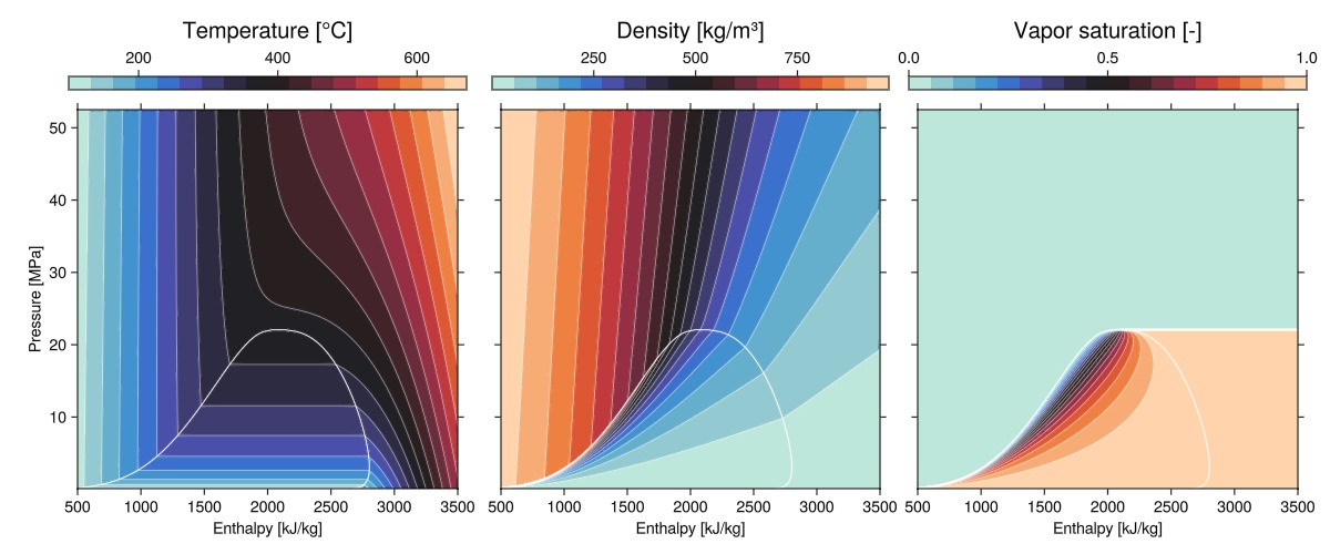
Single-phase benchmark cases
Cases :a to :c remain in the single-phase region for the plotted states. We therefore use them to compare Fimbul and HYDROTHERM pressure and temperature profiles along the 1D column, both with and without gravity.
Case a
Case :a spans 50 to 25 MPa and 350 to 150 °C. The pressure stays high enough that the fluid remains in the compressed-liquid region throughout the column, so the solution is single-phase liquid with smooth pressure and temperature variations.
fig_case_a = plot_case_profiles(:a, all_results)
fig_case_a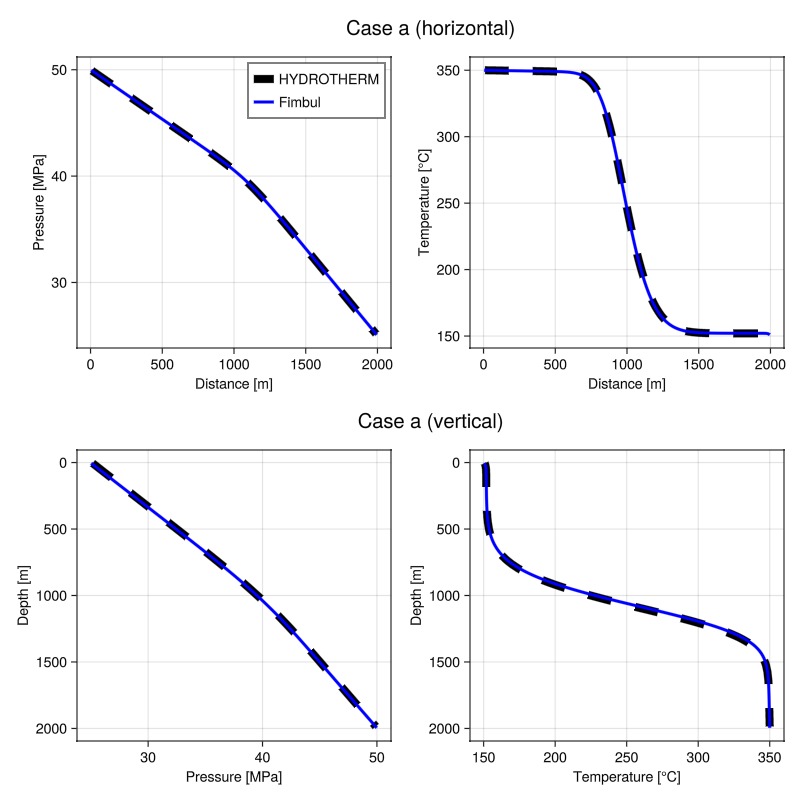
Case b
Case :b spans 40 to 20 MPa and 450 to 300 °C. These conditions are hotter than case :a, but the pressure is still high enough to avoid flashing, so the response remains single-phase while showing stronger thermal contrasts.
fig_case_b = plot_case_profiles(:b, all_results)
fig_case_b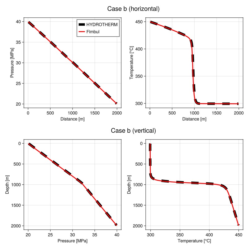
Case c
Case :c spans 15 to 1 MPa and 500 to 350 °C. Here the fluid is much hotter and less compressed, placing it in the vapor-dominated single-phase region, so the profiles represent hot steam rather than liquid water.
fig_case_c = plot_case_profiles(:c, all_results)
fig_case_c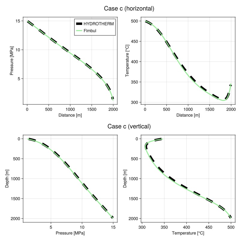
Two-phase benchmark cases
Cases :d and :e traverse the two-phase region. Here we compare Fimbul and HYDROTHERM pressure, temperature, and liquid-saturation profiles, and then compare the no-gravity paths in pressure-enthalpy space.
Case d
Case :d spans 20 to 1 MPa and 400 to 150 °C. The inlet starts as hot, pressurized water, but the strong pressure and temperature drop drives the state path across the saturation envelope, producing a genuine two-phase liquid-vapor transition along the column.
fig_case_d = plot_case_profiles(:d, all_results)
fig_case_d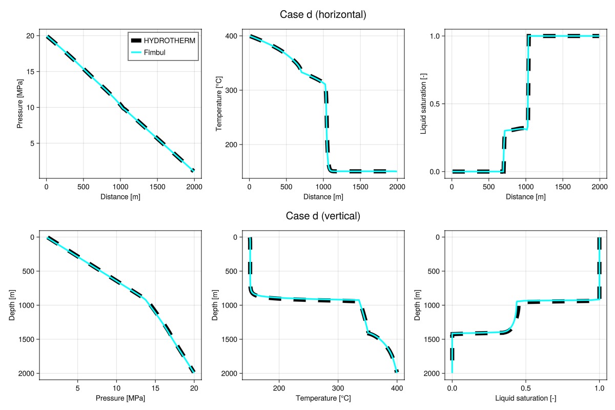
Case e
Case :e spans 4 to 1 MPa and 300 to 150 °C. Because the pressures are low, boiling is easier to trigger than in case :d, so the system develops a broad two-phase region with more pronounced vapor formation.
fig_case_e = plot_case_profiles(:e, all_results)
fig_case_e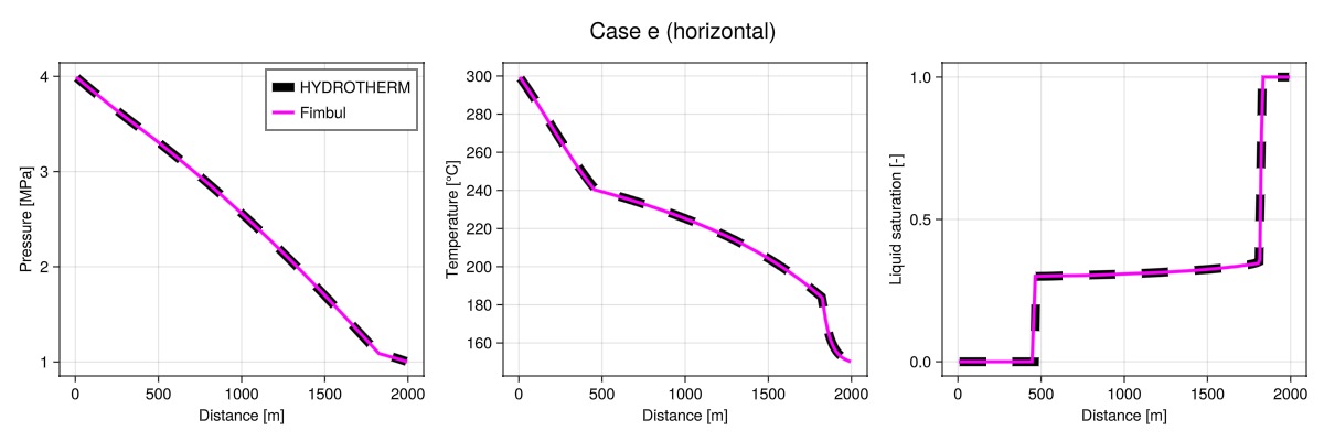
Phase diagram comparison
We compare the horizontal cases directly in pressure-enthalpy space, overlaying Fimbul state paths and HYDROTHERM reference paths on temperature contours.
fig = Figure(size = (700, 640))
Label(fig[0, 1:2], "Phase diagram comparison"; fontsize = 22)
ax = Axis(fig[1, 1]; xticksmirrored = true, yticksmirrored = true, aspect = AxisAspect(1))
handles = Fimbul.plot_phase_diagram_contours!(
    ax,
    tables;
    variable = :temperature,
    pressure_limits = (1e5, 52.5e6),
    enthalpy_limits = (500e3, 3500e3),
    levels = 20,
    lines = true,
)

for case_symbol in (SINGLE_PHASE_CASES..., TWO_PHASE_CASES...)
    hydrotherm = Fimbul.load_hydrotherm_1d_phase_path(case_symbol)
    lines!(ax, hydrotherm.enthalpy_kj_per_kg, hydrotherm.pressure_mpa; linewidth = 6, linestyle = :dash, color = CASE_COLORS[case_symbol])
    out = all_results[(case_symbol, false)]
    state = out.results.states[end]
    Fimbul.plot_reservoir_state_ph!(
        ax,
        state;
        color = CASE_COLORS[case_symbol],
        linewidth = 3,
        label = "Case $(case_symbol)",
    )
end

axislegend(ax; position = :rt)
Colorbar(fig[1, 2], handles.filled, label = "Temperature [°C]")
fig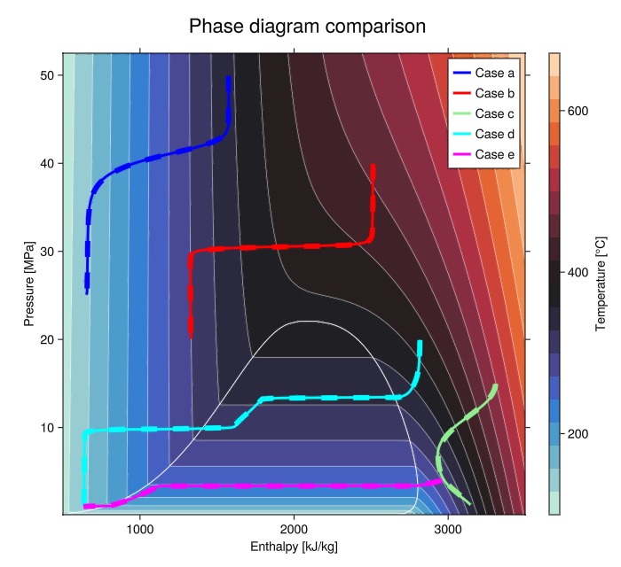
Example on GitHub
If you would like to run this example yourself, it can be downloaded from the Fimbul.jl GitHub repository as a script.
This example took 56.908193171 seconds to complete.This page was generated using Literate.jl.