Three-cycle reactive storage in 2D¶

Follow hydrogen and microbial populations through build-up, injection, idle periods, and withdrawal in a layered storage model. The completed comparison extends to 347.4 days and three storage cycles, with all accepted states retained as packed simulations.

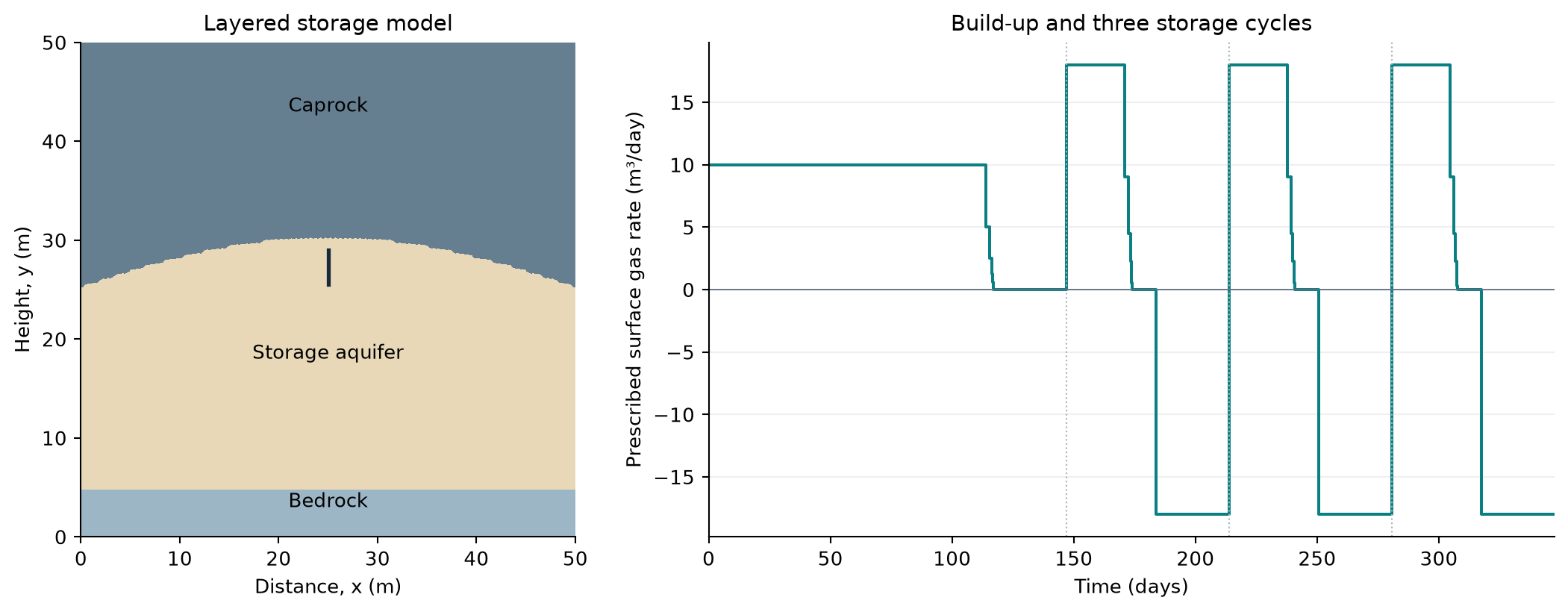
Storage aquifer between caprock and bedrock, with the well and the prescribed build-up and three-cycle gas schedule. — A 50 × 50 m cross-section with 10,116 cells. The well geometry and operating controls come from the existing 2D mineral-coupling example. This is an illustrative layered model, not a calibrated field forecast.¶

Physical setup¶
Region or property	Value
Storage aquifer	Porosity 0.25; permeability 10 mD
Caprock	Porosity 0.10; permeability 0.01 mD
Bedrock	Porosity 0.10; permeability 0.0001 mD
Temperature	317.50 K
Initial salinity	2.865 mol/kg water NaCl
Microbial pathways	Methanogenesis (MET), acetogenesis (ACE), sulfate reduction (SRB)

The paired simulations use compositional thermodynamics and the same grid and well schedule. The baseline solves mobile microbial populations with flow; the coupled case uses cell-local geochemical kinetics and mineral chemistry. Neither enables molecular diffusion, mechanical dispersion, bacterial diffusion, chemotaxis, or bioclogging. The workflow comparison therefore includes changes in kinetic formulation and population transport; it does not isolate mineral chemistry alone.

Explore hydrogen and microbial evolution¶

Choose a workflow, press Play, or move the time slider. Colors retain the same logarithmic limits through time and between workflows. The animation uses selected accepted states, with no interpolated spatial fields.

The hydrogen panel shows liquid-phase H₂ mole fraction, not gas saturation. Population panels show the model population scale relative to its initial value. They make fronts and localized activity visible, but the two kinetic formulations use different biomass representations. Equal colors do not establish equal physical biomass.

In the PHREEQC workflow, populations remain cell-local: spatial changes represent growth and decay. Select the mobile workflow to see aqueous transport together with growth and decay. Neither animation depicts chemotaxis or follows individual bacteria.

Hydrogen consumption and reaction pathways¶

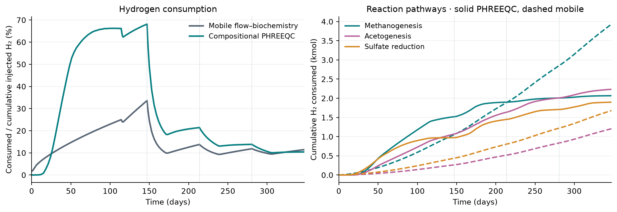
Three-cycle consumed-hydrogen percentage and cumulative metabolic contributions, comparing compositional PHREEQC and mobile flow–biochemistry. — Left: cumulative microbial consumption divided by cumulative prescribed hydrogen injection at each plotted time. Right: MET, ACE and SRB contributions; solid curves use PHREEQC, dashed curves use mobile kinetics. Dotted lines mark the starts of the three storage cycles.¶

The final consumed amounts are 6.199 kmol (10.426%) with compositional PHREEQC and 6.818 kmol (11.466%) with mobile flow–biochemistry. These percentages measure metabolic conversion, excluding dissolved or unrecovered hydrogen. Unlike the 1D validation page, the denominator here grows with cumulative prescribed injection; it is not the final total injection used at every time.

Gas composition and aqueous chemistry¶

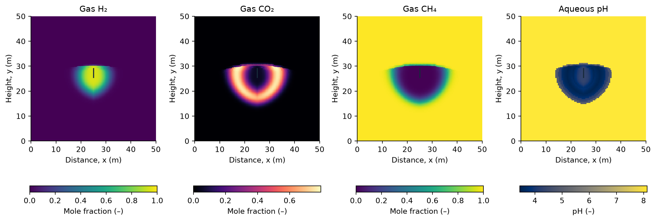
End-of-injection maps of gas-phase H2, CO2 and methane mole fractions, and aqueous pH in the coupled two-dimensional case. — Compositional PHREEQC at the end of the third injection period (day 307.6). Gas compositions are hidden where gas saturation is below 10⁻⁶; pH is shown throughout the aqueous domain. No pressure map is needed to inspect the hydrogen plume and its chemical environment.¶

This selected mineral inventory represents Bentheimer sandstone: 2% dolomite and 98% inert rock by mass, with no initial calcite.

The chemical maps complement the bulk consumption curves: hydrogen exposure, carbon conversion, and pH evolve unevenly around the well. The available per-cell element-audit diagnostics are retained in the result provenance. The coupled result records 62 cell-update audit failures across the three segments, with a maximum absolute residual of 2.68 × 10⁻⁶ mol. The baseline has no equivalent geochemical audit. These counts cover accepted-state diagnostics, not rejected chemistry attempts. The figures do not establish elemental conservation or grid convergence.

Use the existing example¶

startupH2sim('phreeqc', true)
exampleCompositionalBacterial2DPhreeqcMinerals

This is the public entry point for the layered mineral-coupling setup. The displayed three-cycle results are saved continuations of that setup; they are not a claim that the default call reproduces the entire comparison. Save the setup and accepted states with the packed-simulation utilities to retain spatial fields and redraw figures without rerunning chemistry.