Anticlinal hydrogen storage

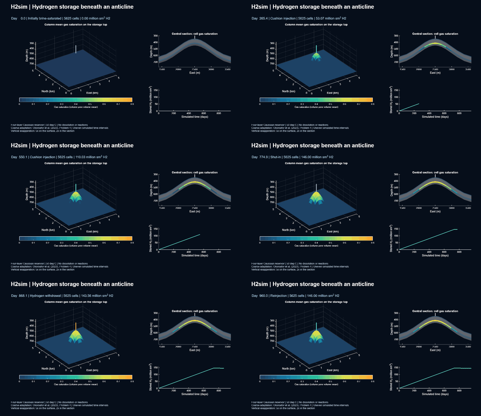
This small three-dimensional case adapts Problem 4 of Okoroafor et al. (2023): a four-layer Gaussian structure with a storage well at its crest. An initially brine-saturated reservoir receives cushion hydrogen, rests during shut-in, and then alternates withdrawal and reinjection. This page combines an animation with figures drawn from the same saved simulation.

Black-oil flow · Four geological layers · 5625 cells · No PHREEQC required

The left panel drapes pore-volume-weighted column gas saturation over the storage formation’s top surface; it is not an isosurface or the top cell’s saturation. The central vertical section shows cell gas saturations above 0.005 against the four geological layers. The history panel shows hydrogen inventory in surface cubic metres. Both saturation panels use fixed color limits from zero to 0.8. Vertical exaggeration is fivefold on the 3D surface and twofold in the section. For this preview, up to 160 initial/accepted states are selected by physical time, retaining every operating-stage endpoint, without temporal interpolation. Labelled simulation times are uneven; playback is not real time.

Download the MP4, GIF or provenance record.

Geological structure

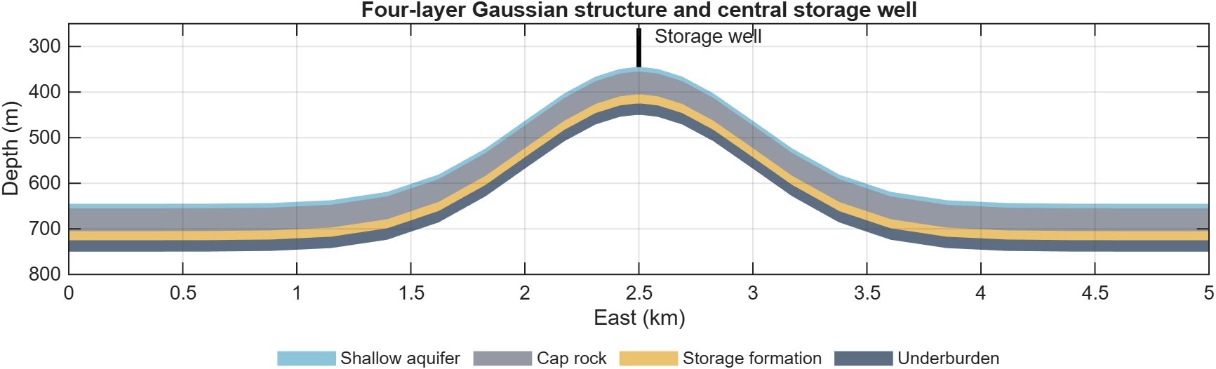
Geological layers and the central well. The well fully penetrates the 20 m storage formation. Depth increases downward; vertical exaggeration is twofold. Layer properties are listed below.

Download vector PDF.

Plume development

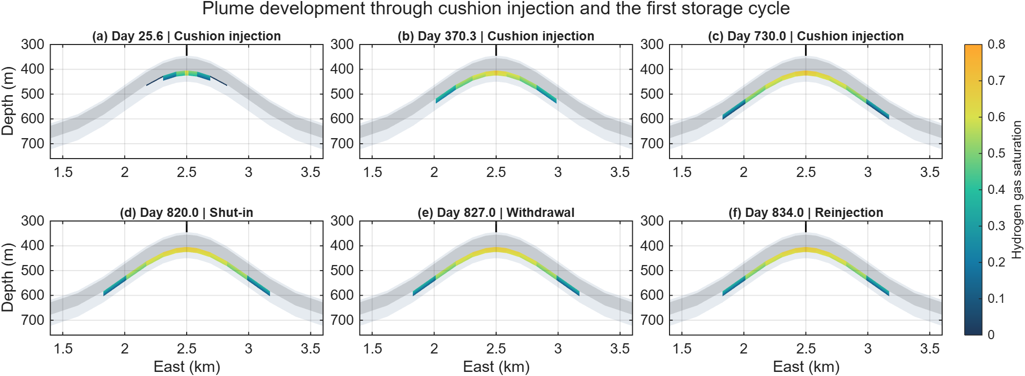
Gas migration through cushion injection, shut-in and the first storage cycle. Every panel uses the same saturation scale. Labels show actual accepted-state times, nearest the requested milestones. Cells below 0.005 gas saturation are hidden; sections have twofold vertical exaggeration.

Download vector PDF.

Operating response and ten storage cycles

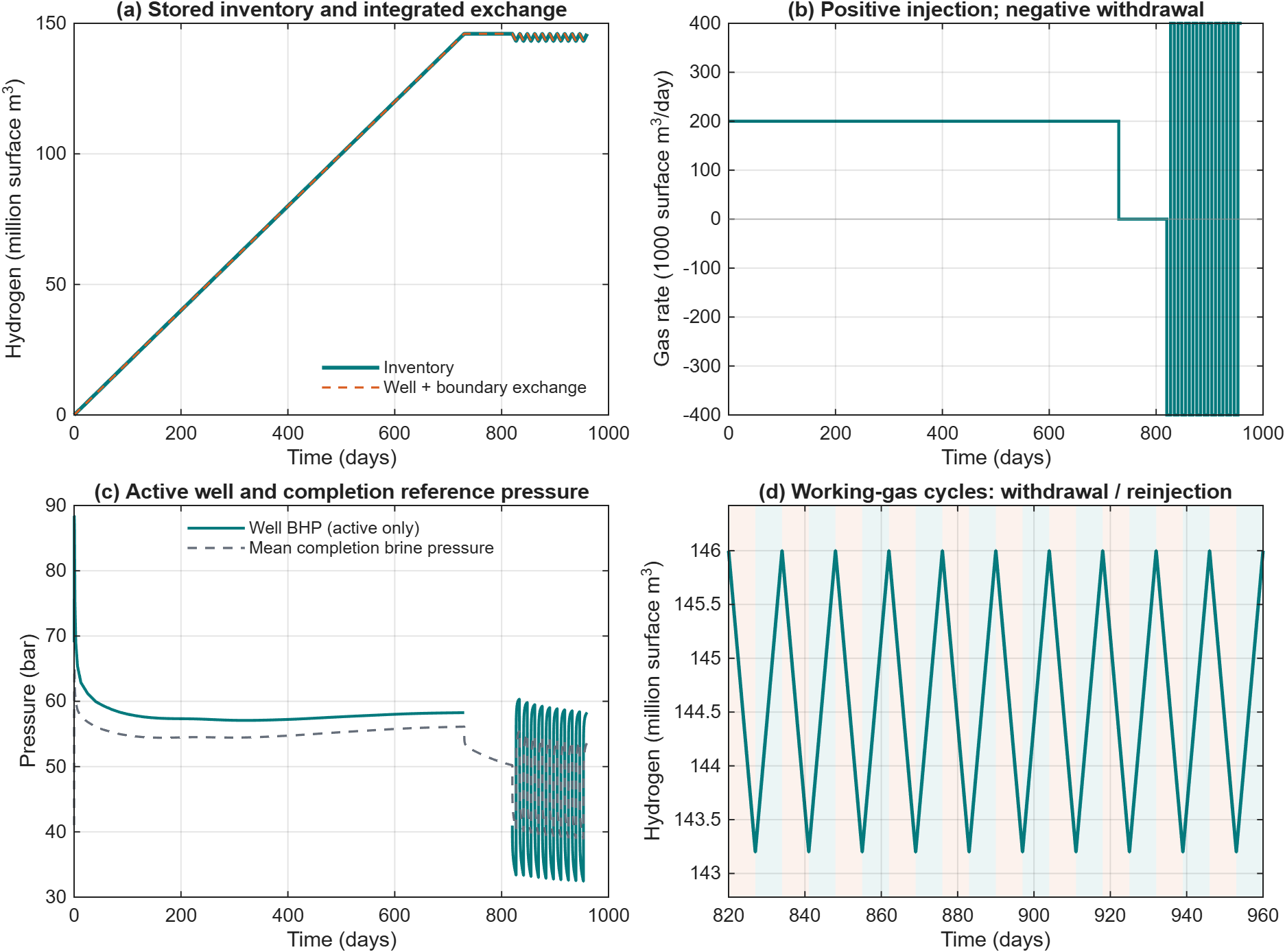
Stored hydrogen agrees with integrated well and boundary exchange. Positive gas rate is injection; negative rate is withdrawal. Inactive-well BHP is omitted, while the mean saved brine-phase pressure in the completion cells remains visible. The cycle close-up shows all ten withdrawal/reinjection pairs: orange shading marks withdrawal and teal shading marks reinjection. Inventory is reported at the stated surface reference conditions.

Download vector PDF. The figure provenance records the source states and export hashes. These are simulation figures, not measurements or external benchmark comparison curves.

Run the example

This example was added after v0.1.0. Use a development checkout containing exampleHydrogenAnticline. Supplementary previews on the release page do not change the original version tag’s source files.

startupH2sim
result = exampleHydrogenAnticline('buildupDays', 730, 'numCycles', 10);
animateHydrogenAnticline(result, fullfile('build', 'anticline'), ...
    'frameRate', 6, 'maxFrames', 160);

The simulation creates no files or figures. Save the result once to redraw it:

plotHydrogenAnticline(result, 'outputDirectory', fullfile('build', 'anticline'));
save('anticlineResults.mat', 'result', '-v7');
load('anticlineResults.mat', 'result');
animateHydrogenAnticline(result, fullfile('build', 'anticline'), ...
    'frameRate', 6, 'maxFrames', 160);

A smaller complete-operation check uses:

small = exampleHydrogenAnticline('horizontalCells', [9, 9], ...
    'buildupDays', 90, 'shutInDays', 20, 'numCycles', 1);

This shorter case does not reproduce the displayed extended run. PHREEQC, external fluid-data downloads and Parallel Computing Toolbox are unnecessary. MP4 requires MATLAB’s MPEG-4 VideoWriter profile. Pass 'writeVideo', false to the renderer on platforms without that profile to export GIF and PNG only.

Geometry and operation

The domain is 5 km by 5 km, with a 105 m stratigraphic thickness. The base horizon follows

\[z_b = 750 - 300\exp\left[-\frac{(x-2500)^2+(y-2500)^2}{2(500)^2}\right].\]

Layer tops follow this shape. The analytical top of the storage formation is 405 m deep at the crest. Discrete cell corners approximate the curved surface; coarse grids therefore have a slightly deeper crest. The default grid has 25 by 25 horizontal cells clustered toward the centre and nine vertical cells, for 5625 cells. Four central well completions span the storage formation.

Layer properties, from shallow to deep

Layer	Thickness (m)	Porosity	Permeability (m²)	Entry pressure (MPa)
Shallow aquifer	10	0.1	9.87e-15	0.4
Cap rock	50	0.1	9.87e-20	4
Storage formation	20	0.25	6.91e-13	0.4
Underburden	25	0.1	9.87e-18	4

The default schedule injects 200,000 surface m³/day for 365 days, shuts the well for 90 days, then performs five cycles of seven days of withdrawal and seven days of reinjection at 400,000 surface m³/day. Withdrawal controls the gas rate; reinjection is pure hydrogen. The default total duration is 525 days. The displayed preview extends cushion injection to 730 days, retaining the same rates and 90-day shut-in, and uses ten storage cycles, for a total of 960 days. This injects twice the cushion volume and allows the resolved plume to spread farther. At the end of cushion injection, the resolved plume radius at a cell gas saturation of at least 0.05 grows from approximately 429 m in the default run to 596 m in the extended run. This is a grid-dependent extent measure. The extension is an illustration variant, not the published benchmark schedule. Ramp timesteps preserve every stage duration. Hydrostatic pressure conditions apply on all four lateral sides; top and bottom are sealed. Initial brine pressure is 4.1 MPa at 415 m depth, and temperature is fixed at 323.15 K.

Model choices and limits

This implementation uses H2sim’s black-oil workflow with brine in phase O and hydrogen in phase G. Hydrogen density uses the local Brill–Beggs correlation; brine reference density is 1000 kg/m³ with compressibility 4.5e-10 Pa⁻¹. Constant viscosities are 0.55 mPa s for brine and 9 µPa s for hydrogen. Surface reference conditions are 288.71 K and 101325 Pa. Rock compressibility is 1.5e-12 Pa⁻¹. These are explicit fluid approximations, not the original paper’s complete PVT specification.

Relative permeabilities use the published endpoints and exponents. The Brooks–Corey capillary curve uses index 1.2, with a minimum effective water saturation of 1e-3 to keep the entry-pressure function finite. Dissolution, water vaporization, hysteresis and microbial reactions are disabled. The warped grid uses TPFA; this coarse demonstration is not a grid-convergence study or an external benchmark validation.

The example checks positive finite pressures, normalized bounded saturations and hydrogen inventory against integrated active-well and pressure-boundary surface gas fluxes, with a 1e-5 relative balance bound. Inactive-well rates are excluded explicitly. H2StoreAnticlineExampleTest checks layer properties, completions, exact stage totals, fluid functions, prescribed gas-volume exchange, well-rate signs, public inventory accounting, input errors and animation export. Run it through runH2StoreTests as described in Local verification.

Source: Okoroafor et al. (2023), Problem 4 and Table 8. The public benchmark data repository is MIT-licensed. This independent implementation regenerates the analytical geometry and does not bundle the original grid or reference output. New H2sim source uses the project’s GPL-3.0-or-later notice.