Gradients at cyclic steady state

This example computes how the performance of the four-stage VSA cycle of Haghpanah et al. (2013) at cyclic steady state changes with its operating settings: the feed velocity, the blowdown and evacuation pressures, and the durations of the four stages. These are the gradients an optimiser needs, and here they come from adjoints rather than from re-running the cycle to steady state once per setting.

The cycle maps its initial state x to its final state Φ(x, p), where p holds the settings. Cyclic steady state is the fixed point x* = Φ(x*, p), which moves when p changes. For an objective J over one cycle, the implicit function theorem gives

dJ/dp = ∂J/∂p + μᵀ ∂Φ/∂p,   where   (I − ∂Φ/∂x)ᵀ μ = ∂J/∂x.

Every term comes from adjoint solves over a single cycle: GMRES finds μ from products with (∂Φ/∂x)ᵀ, and a last adjoint gives the derivatives with respect to all parameters and stage settings together.

import Mocca
using Mocca.Units
using CairoMakie

1. The process and its design variables

The four-stage VSA process with 30 cells. Each stage starts with short steps (first_dt, the default). Without them, the 1 s step at the abrupt start of a stage can converge to a slightly different solution for a slightly different start, and the cycle map jumps. A gradient of a map that jumps is meaningless.

process = Mocca.four_stage_vsa_process(ncells = 30)

Process four-stage VSA: CO2/N2 feed at 1.0 bar, 298.15 K, capturing CO2
  Bed: fixed bed of zeolite 13X, 30 cells
    bottom V_feed (feed), from boundary at 1.0 bar; V_vacuum (extract), to boundary at 0.1 bar
    top    V_product (product), to boundary at 1.0 bar
  cycle of 4 stages, 100.0 s:
    pressurisation                        15.0 s   V_feed
    adsorption                            15.0 s   V_feed, V_product
    blowdown                              30.0 s   V_product
    evacuation                            40.0 s   V_vacuum

A design variable names the places it sets. Pressures carry over from step to step, so one place is enough for each: the evacuation pressure is also where the next pressurisation starts. Since durations are among the variables, a stage of a different duration keeps the steps it has now, stretched in proportion, which is what the duration gradients describe.

Mocca.add_variable!(process, :v_feed, ("adsorption", :velocity))
Mocca.add_variable!(process, :P_L, ("evacuation", :to))
Mocca.add_variable!(process, :P_I, ("blowdown", :to))
Mocca.add_variable!(process, :t_press, ("pressurisation", :duration))
Mocca.add_variable!(process, :t_ads, ("adsorption", :duration))
Mocca.add_variable!(process, :t_blow, ("blowdown", :duration))
Mocca.add_variable!(process, :t_evac, ("evacuation", :duration))
process

Process four-stage VSA: CO2/N2 feed at 1.0 bar, 298.15 K, capturing CO2
  Bed: fixed bed of zeolite 13X, 30 cells
    bottom V_feed (feed), from boundary at 1.0 bar; V_vacuum (extract), to boundary at 0.1 bar
    top    V_product (product), to boundary at 1.0 bar
  cycle of 4 stages, 100.0 s:
    pressurisation                        15.0 s   V_feed
    adsorption                            15.0 s   V_feed, V_product
    blowdown                              30.0 s   V_product
    evacuation                            40.0 s   V_vacuum
  variables: v_feed, P_L, P_I, t_press, t_ads, t_blow, t_evac

2. Performance and its gradient at cyclic steady state

performance_gradient finds the steady state (a few plain cycles, then Newton's method on the cycle map, with its Jacobian from forward sensitivities over one cycle) and then the gradients. The gradient is only as accurate as the steady state, since the slowest mode of this cycle decays by only about 1% per cycle. Purity, recovery, energy and productivity are ratios of sums over the cycle (the CO₂ and the gas in the extract, the CO₂ fed, the pump and compressor work), and their gradients follow by the quotient rule.

g = Mocca.performance_gradient(process)
metrics = g.metrics[(:purity, :recovery, :specific_energy, :productivity)]
for (k, v) in pairs(metrics)
    println(rpad(k, 18), round(v, sigdigits = 4))
end

purity            0.7951
recovery          0.3668
specific_energy   141.3
productivity      0.2366

Relative sensitivities, (x/J) dJ/dx: the percentage change in each metric for a 1% change in each setting.

names = Mocca.variable_names(process)
println(rpad("", 10), join([rpad(k, 18) for k in keys(metrics)]))
for n in names
    println(rpad(n, 10), join([rpad(round(process[n] * g.gradients[m][n] / metrics[m], sigdigits = 3), 18) for m in keys(metrics)]))
end

          purity            recovery          specific_energy   productivity
v_feed    0.14              -0.347            -0.21             0.49
P_L       -0.0859           -1.75             0.468             -1.84
P_I       -0.323            0.529             -0.523            0.533
t_press   0.00267           0.0113            -0.00721          -0.138
t_ads     0.16              -0.227            -0.306            0.447
t_blow    -0.0051           -0.0194           0.0553            -0.319
t_evac    0.00335           0.0268            -0.00458          -0.372

3. Check against finite differences

Change the feed velocity and the adsorption time by ±0.01%, converge each case to steady state with Newton's method from the last steady state, and difference the metrics.

for n in (:v_feed, :t_ads)
    x0 = process[n]
    h = 1e-4 * x0
    process[n] = x0 + h
    up = Mocca.performance(process; tol = 1e-10)
    process[n] = x0 - h
    down = Mocca.performance(process; tol = 1e-10)
    process[n] = x0
    println(n)
    for k in keys(metrics)
        fd = (up[k] - down[k]) / 2h
        println("  ", rpad(k, 18), "adjoint ", round(g.gradients[k][n], sigdigits = 8), "   finite difference ", round(fd, sigdigits = 8))
    end
end

v_feed
  purity            adjoint 0.11110539   finite difference 0.1111054
  recovery          adjoint -0.12712426   finite difference -0.12712426
  specific_energy   adjoint -29.616429   finite difference -29.616431
  productivity      adjoint 0.1159269   finite difference 0.1159269
t_ads
  purity            adjoint 0.008474888   finite difference 0.0084748881
  recovery          adjoint -0.0055527978   finite difference -0.0055527977
  specific_energy   adjoint -2.8800388   finite difference -2.8800389
  productivity      adjoint 0.0070545494   finite difference 0.0070545495

4. Relative sensitivities

Each bar is an elasticity: the percentage change of a measure for a 1% increase of a setting, from the gradients above. The evacuation pressure P_L matters most: 1% lower raises recovery by almost 2% and productivity by about as much, and lowers the energy per tonne by about 0.5%. Purity responds most to the blowdown pressure P_I.

fig = Figure(size = (1100, 340))
for (j, m) in enumerate(keys(metrics))
    ax = Axis(fig[1, j], title = String(m), xticks = (1:length(names), String.(names)),
        xticklabelrotation = π / 6, ylabel = j == 1 ? "% change per 1% change" : "")
    vals = [process[n] * g.gradients[m][n] / metrics[m] for n in names]
    barplot!(ax, 1:length(vals), vals)
    hlines!(ax, [0.0], color = :black, linewidth = 0.5)
end
fig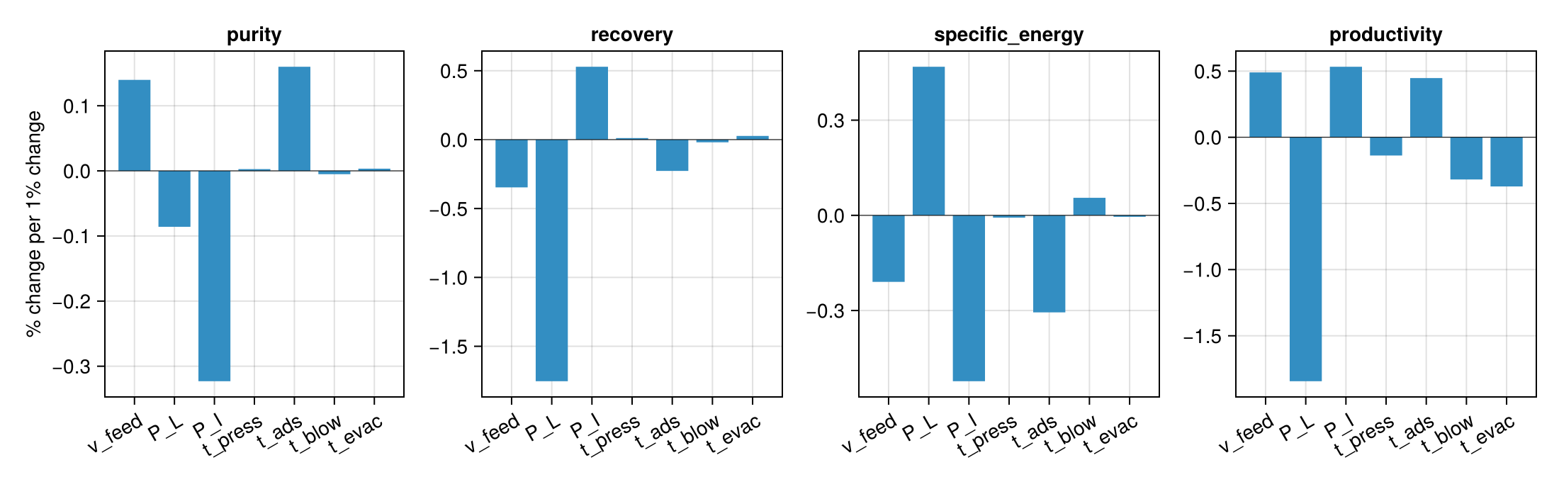

Example on GitHub

If you would like to run this example yourself, it can be downloaded from the Mocca.jl GitHub repository.

---

This page was generated using Literate.jl.