A fully differentiable geothermal doublet: History matching and control optimization

Geothermal   StartToFinish   Advanced   HistoryMatching   Optimization   Differentiability  

We are going to set up a conceptual geothermal doublet model in 2D and perform gradient based history matching. This example serves two main purposes:

1. It demonstrates the conceptual workflow for setting up a geothermal model from scratch with a fairly straightforward mesh setup.

2. It shows how to set up a gradient based history matching workflow with the generic optimization interface that allows for optimizing any input parameter used in the setup of a model.

Load packages and define units

using Jutul, JutulDarcy, GLMakie
meter, kilogram, bar, year, liter, second, darcy, day = si_units(:meter, :kilogram, :bar, :year, :liter, :second, :darcy, :day)

(1.0, 1.0, 100000.0, 3.1556952e7, 0.001, 1.0, 9.86923266716013e-13, 86400.0)

Set up the reservoir mesh

The model is a typical geothermal case where there is a layer of high permeability in the middle, confined between two low-permeable layers. For a geothermal model, the low permeable layers are important, as they store significant amounts of heat that can be conducted to the high permeable layer during production.

We set up the mesh so that the high permeable layer where most of the advective transport occurs has a higher lateral resolution than the low permeable layers. The model is also essentally 2D as there is only one cell thickness in the y direction - a choice that is made to make the example fast to run, especially during the later optimization stages where many simulations must be run to achieve convergence.

nx = 50
ntop = 5
nmiddle = 10
nbottom = 5
nz = ntop + nmiddle + nbottom

20

Set up layer thicknesses and vertical cell thicknesses

top_layer_thickness = 300.0*meter
middle_layer_thickness = 200.0*meter
bottom_layer_thickness = 300.0*meter
dz = Float64[]
for i in 1:ntop
    push!(dz, top_layer_thickness/ntop)
end
for i in 1:nmiddle
    push!(dz, middle_layer_thickness/nmiddle)
end
for i in 1:ntop
    push!(dz, bottom_layer_thickness/nbottom)
end

rmesh = reservoir_mesh((nx, 1, nz), (2000.0, 50.0, dz))

UnstructuredMesh with 1000 cells, 1930 faces and 2140 boundary faces

Define regions based on our selected depths

We tag each cell with a region number based on its depth. The top layer is region 1, the middle layer is region 2, and the bottom layer is region 3.

geo = tpfv_geometry(rmesh)
depths = geo.cell_centroids[3, :]
regions = Int[]
for (i, d_i) in enumerate(depths)
    if d_i <= top_layer_thickness
        r = 1
    elseif d_i <= top_layer_thickness + middle_layer_thickness
        r = 2
    else
        r = 3
    end
    push!(regions, r)
end

Plot the mesh and regions

fig, ax, plt = plot_cell_data(rmesh, regions,
    alpha = 0.5,
    outer = true,
    transparency = true,
    colormap = Categorical(:heat)
)
ax.elevation[] = 0.0
ax.azimuth[] = π/2
plot_mesh_edges!(ax, rmesh)
fig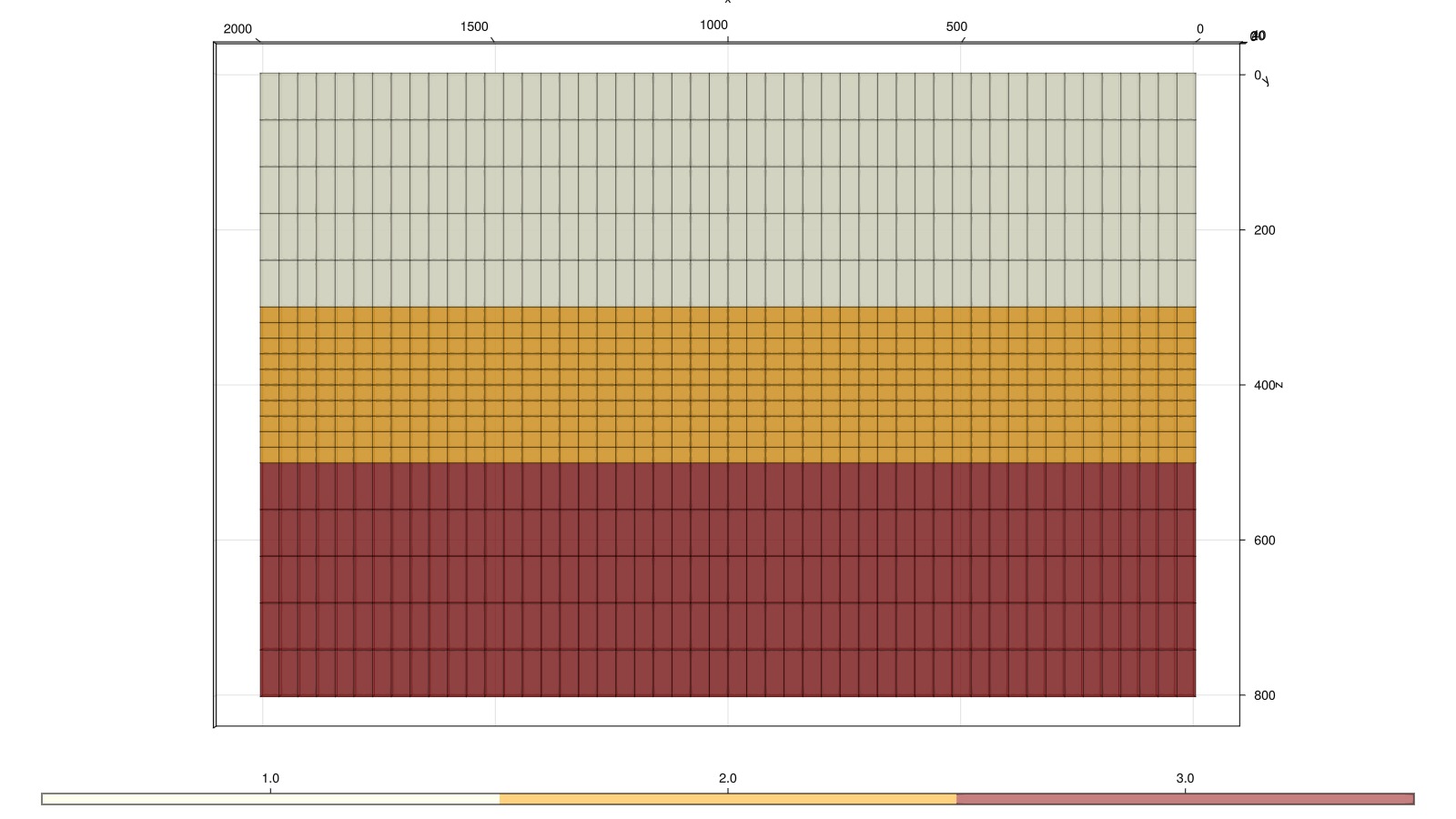

Define functions for setting up the simulation

We will define a function that takes in a Dict with different values and sets up the simulation. The key idea is that we can then optimize the values in the Dict to perform optimization. As we can define any such Dict to set up the model, this interface is very flexible and can be used for both control optimization and history matching with respect to almost any parameter of the model. The disadvantage is that the setup function will be called many times, which can be a substantial cost compared to the more structured optimization interface that only allows for optimization of the numerical parameters (e.g. for the CGNet example).

Define the time schedule

We set up a time schedule for the simulation. The total simulation time is 30 years, and we report the results every 120 days. We also define ten different intervals in this 30 year period, which are the period where we will allow the rates and temperatures to vary during the last part of the optimization tutorial.

total_time = 30.0*year
report_step_length = 120.0*day
dt = fill(report_step_length, Int(ceil(total_time/report_step_length)))
num_intervals = 10
interval_interval = total_time/num_intervals
interval_for_step = map(t -> min(Int(ceil(t/interval_interval)), num_intervals), cumsum(dt))

92-element Vector{Int64}:
  1
  1
  1
  1
  1
  1
  1
  1
  1
  2
  ⋮
 10
 10
 10
 10
 10
 10
 10
 10
 10

Define the wells

We set up two wells, one injector and one producer. The injector is located at the left side of the model, and the producer is located at the right side. We use multisegment wells.

base_rate = 15*liter/second
base_temp = 15.0

domain = reservoir_domain(rmesh)
inj_well = setup_vertical_well(domain, 5, 1,
    heel = ntop+1,
    toe = ntop+nmiddle,
    name = :Injector,
    simple_well = false
)
prod_well = setup_vertical_well(domain, nx - 5, 1,
    heel = ntop+1,
    toe = ntop+nmiddle,
    name = :Producer,
    simple_well = false
)

model_base = setup_reservoir_model(
    domain, :geothermal,
    wells = [inj_well, prod_well],
);

Set up a helper to define the forces for a given rate and temperature

function setup_doublet_forces(model, inj_temp, inj_rate)
    T_Kelvin = convert_to_si(inj_temp, :Celsius)
    rate_target = TotalRateTarget(inj_rate)
    ctrl_inj  = InjectorControl(rate_target, [1.0],
        density = 1000.0, temperature = T_Kelvin)

    bhp_target = BottomHolePressureTarget(50*bar)
    ctrl_prod = ProducerControl(bhp_target)

    control = Dict(:Injector => ctrl_inj, :Producer => ctrl_prod)
    return setup_reservoir_forces(model, control = control)
end

setup_doublet_forces (generic function with 1 method)

Define the main setup function

This function sets up the model based on the parameters provided in the Dict. It takes in two arguments: The required parameters in a Dict and an optional step_info argument that can be used to set up the model for a specific time step. The function returns a JutulCase object that can be used to simulate the reservoir. Here, we ignore the step_info argument and set up the entire schedule every time. Jutul will then automatically use the correct force based on the time step in the simulation.

function setup_doublet_case(prm, step_info = missing)
    model = deepcopy(model_base)
    rdomain = reservoir_domain(model)
    rdomain[:permeability] = prm["layer_perm"][regions]
    rdomain[:porosity] = prm["layer_porosities"][regions]
    rdomain[:rock_heat_capacity] = prm["layer_heat_capacity"][regions]

    T0 = convert_to_si(70, :Celsius)
    thermal_gradient = 20.0/1000.0*meter
    eql = EquilibriumRegion(model, 50*bar, 0.0, temperature_vs_depth = z -> T0 + z*thermal_gradient)
    state0 = setup_reservoir_state(model, eql)

    forces_per_interval = map((T, rate) -> setup_doublet_forces(model, T, rate),
        prm["injection_temperature_C"], prm["injection_rate"])

    forces = forces_per_interval[interval_for_step]

    return JutulCase(model, dt, forces, state0 = state0)
end

setup_doublet_case (generic function with 2 methods)

Perform a history match

We first set up a truth case that we will use to generate the data for the history match. We define high perm and porosity in the middle layer, and low perm and porosity in the top and bottom layers before simulating the model.

prm_truth = Dict(
    "injection_rate" => fill(base_rate, num_intervals),
    "injection_temperature_C" => fill(base_temp, num_intervals),
    "layer_porosities" => [0.1, 0.3, 0.1],
    "layer_perm" => [0.01, 0.8, 0.02].*darcy,
    "layer_heat_capacity" => [500.0, 600.0, 450.0], # Watt / m K
)
case_truth = setup_doublet_case(prm_truth)
ws, states = simulate_reservoir(case_truth)

ReservoirSimResult with 92 entries:

  wells (2 present):
    :Producer
    :Injector
    Results per well:
       :lrat => Vector{Float64} of size (92,)
       :wrat => Vector{Float64} of size (92,)
       :temperature => Vector{Float64} of size (92,)
       :control => Vector{Symbol} of size (92,)
       :Aqueous_mass_rate => Vector{Float64} of size (92,)
       :bhp => Vector{Float64} of size (92,)
       :wcut => Vector{Float64} of size (92,)
       :mass_rate => Vector{Float64} of size (92,)
       :rate => Vector{Float64} of size (92,)
       :mrat => Vector{Float64} of size (92,)

  states (Vector with 92 entries, reservoir variables for each state)
    :Pressure => Vector{Float64} of size (1000,)
    :TotalMasses => Matrix{Float64} of size (1, 1000)
    :TotalThermalEnergy => Vector{Float64} of size (1000,)
    :FluidEnthalpy => Matrix{Float64} of size (1, 1000)
    :Temperature => Vector{Float64} of size (1000,)
    :PhaseMassDensities => Matrix{Float64} of size (1, 1000)
    :RockInternalEnergy => Vector{Float64} of size (1000,)
    :FluidInternalEnergy => Matrix{Float64} of size (1, 1000)

  time (report time for each state)
     Vector{Float64} of length 92

  result (extended states, reports)
     SimResult with 92 entries

  extra
     Dict{Any, Any} with keys :simulator, :config

  Completed at Jul. 02 2026 16:39 after 5 seconds, 29 milliseconds, 792.4 microseconds.

Define a mismatch objective function

The mismatch objective function is defined as the sum of squares difference between the simulated values and the reference values observed in the wells. Note that we only make use of the well data:

• The temperature at the producer well

• The mass rate at the producer well (since it is controlled on BHP)

• The BHP at the injector well (since it is controlled on rate)

We use the get_1d_interpolator function to create interpolators for the reference values, since we cannot assume that the simulator will use exactly the same time-steps as the reference values.

prod_rate = ws.wells[:Producer][:wrat]
prod_temp = ws.wells[:Producer][:temperature]
inj_bhp = ws.wells[:Injector][:bhp]

prod_temp_by_time = get_1d_interpolator(ws.time, prod_temp)
prod_rate_by_time = get_1d_interpolator(ws.time, prod_rate)
inj_pressure_by_time = get_1d_interpolator(ws.time, inj_bhp)

import JutulDarcy: compute_well_qoi
function mismatch_objective(m, s, dt, step_info, forces)
    current_time = step_info[:time]
    # Current values
    T_at_prod = compute_well_qoi(m, s, forces, :Producer, :temperature)
    rate = compute_well_qoi(m, s, forces, :Producer, :wrat)
    bhp = compute_well_qoi(m, s, forces, :Injector, :bhp)
    # Reference values
    T_at_prod_ref = prod_temp_by_time(current_time)
    rate_ref = prod_rate_by_time(current_time)
    bhp_ref = inj_pressure_by_time(current_time)
    # Define mismatch by scaling each term
    T_mismatch = (T_at_prod_ref - T_at_prod)
    rate_mismatch = (rate_ref - rate)*1000
    bhp_mismatch = (bhp - bhp_ref)/bar
    return dt * sqrt(T_mismatch^2 + rate_mismatch^2 + bhp_mismatch^2) / total_time
end

mismatch_objective (generic function with 1 method)

Pick an initial guess

We set up an initial guess for the parameters that we will optimize. We assume the injection rate and temperature to be known and we set the porosities and permeabilities to uniform values. The heat capacity is given a bit of layering, but still with completely wrong values.

prm_guess = Dict(
    "injection_rate" => fill(base_rate, num_intervals),
    "injection_temperature_C" => fill(base_temp, num_intervals),
    "layer_porosities" => [0.2, 0.2, 0.2],
    "layer_perm" => [0.2, 0.2, 0.2].*darcy,
    "layer_heat_capacity" => [400.0, 400.0, 400.0]
)
case_guess = setup_doublet_case(prm_guess)
ws_guess, states_guess = simulate_reservoir(case_guess)

ReservoirSimResult with 92 entries:

  wells (2 present):
    :Producer
    :Injector
    Results per well:
       :lrat => Vector{Float64} of size (92,)
       :wrat => Vector{Float64} of size (92,)
       :temperature => Vector{Float64} of size (92,)
       :control => Vector{Symbol} of size (92,)
       :Aqueous_mass_rate => Vector{Float64} of size (92,)
       :bhp => Vector{Float64} of size (92,)
       :wcut => Vector{Float64} of size (92,)
       :mass_rate => Vector{Float64} of size (92,)
       :rate => Vector{Float64} of size (92,)
       :mrat => Vector{Float64} of size (92,)

  states (Vector with 92 entries, reservoir variables for each state)
    :Pressure => Vector{Float64} of size (1000,)
    :TotalMasses => Matrix{Float64} of size (1, 1000)
    :TotalThermalEnergy => Vector{Float64} of size (1000,)
    :FluidEnthalpy => Matrix{Float64} of size (1, 1000)
    :Temperature => Vector{Float64} of size (1000,)
    :PhaseMassDensities => Matrix{Float64} of size (1, 1000)
    :RockInternalEnergy => Vector{Float64} of size (1000,)
    :FluidInternalEnergy => Matrix{Float64} of size (1, 1000)

  time (report time for each state)
     Vector{Float64} of length 92

  result (extended states, reports)
     SimResult with 92 entries

  extra
     Dict{Any, Any} with keys :simulator, :config

  Completed at Jul. 02 2026 16:39 after 775 milliseconds, 534 microseconds, 288 nanoseconds.

Set up the optimization

We define a dictionary optimization problem that will optimize the parameters in the prm_guess dictionary. We start by setting up the object itself, which takes in the initial guess Dict and the corresponding setup function.

opt = JutulDarcy.setup_reservoir_dict_optimization(prm_guess, setup_doublet_case)

DictParameters with 5 parameters (0 active), and 0 multipliers:
No active optimization parameters.
Inactive optimization parameters
┌─────────────────────────┬──────────────────┬───────┬─────┬─────┐
│                    Name │ Initial value    │ Count │ Min │ Max │
├─────────────────────────┼──────────────────┼───────┼─────┼─────┤
│     layer_heat_capacity │ 400.0 ± 0.0      │     3 │   - │   - │
│          injection_rate │ 0.015 ± 3.47e-18 │    10 │   - │   - │
│ injection_temperature_C │ 15.0 ± 0.0       │    10 │   - │   - │
│              layer_perm │ 1.97e-13 ± 0.0   │     3 │   - │   - │
│        layer_porosities │ 0.2 ± 2.78e-17   │     3 │   - │   - │
└─────────────────────────┴──────────────────┴───────┴─────┴─────┘
No multipliers set.

Define active parameters and their limits

Note that while the parameters get listed, they are all marked as inactive. We need to explicitly make them free/active and specify a range for each parameter before we can optimize them. We use wide absolute limits for each entry.

free_optimization_parameter!(opt, "layer_perm", abs_max = 1.5*darcy, abs_min = 0.01*darcy)
free_optimization_parameter!(opt, "layer_heat_capacity", abs_max = 1000.0, abs_min = 400.0)
free_optimization_parameter!(opt, "layer_porosities", abs_max = 0.35, abs_min = 0.05)

DictParameters with 5 parameters (3 active), and 0 multipliers:
Active optimization parameters
┌─────────────────────┬────────────────┬───────┬──────────┬──────────┐
│                Name │ Initial value  │ Count │      Min │      Max │
├─────────────────────┼────────────────┼───────┼──────────┼──────────┤
│          layer_perm │ 1.97e-13 ± 0.0 │     3 │ 9.87e-15 │ 1.48e-12 │
│ layer_heat_capacity │ 400.0 ± 0.0    │     3 │    400.0 │   1000.0 │
│    layer_porosities │ 0.2 ± 2.78e-17 │     3 │     0.05 │     0.35 │
└─────────────────────┴────────────────┴───────┴──────────┴──────────┘
Inactive optimization parameters
┌─────────────────────────┬──────────────────┬───────┬─────┬─────┐
│                    Name │ Initial value    │ Count │ Min │ Max │
├─────────────────────────┼──────────────────┼───────┼─────┼─────┤
│          injection_rate │ 0.015 ± 3.47e-18 │    10 │   - │   - │
│ injection_temperature_C │ 15.0 ± 0.0       │    10 │   - │   - │
└─────────────────────────┴──────────────────┴───────┴─────┴─────┘
No multipliers set.

Call the optimizer

Now that we have freed a few parameters, we can call the optimizer with the objective function. The defaults for the optimizer are fairly reasonable, so we do not tweak the convergence criteria or the maximum number of iterations. Note that by default the optimizer uses LBFGS, but it is also possible to pass other optimizers as a callable function. Here we use the optimizer lbfgs_qp. By default, this optimizer does no parameter scaling, but since our parameters span a wide range of magnitudes (perm ~ O(10^-15) and heat capacity ~ O(10^3)), this can lead to numerical issues. By passing scale = true the optimizer will effectively scale all parameters to [0, 1] and transform the optimization problem, avoiding numerical issues.

prm_opt = JutulDarcy.optimize_reservoir(opt, mismatch_objective, max_it = 50, gradient_scaling = false, optimizer = :lbfgsb_qp, scale = true);

Optimization: Starting calibration of 9 parameters.
Jutul: Simulating 30 years, 11.82 weeks as 92 report steps
Optimization: Setting up adjoint storage.
Optimization: Finished setup in 70.467938633 seconds.
Optimization: Adjoint solve took 40.558612398 seconds.

Optimization: Objective #1: 1.81476e+01, gradient 2-norm: 8.40764e+12
It:  0 | v: 1.815e+01 | ls-its:  0 | pg: 1.18e+01 | ρ:       NaN | qp-its:  0 +  0 | n-active:   0
Jutul: Simulating 30 years, 11.82 weeks as 92 report steps
Optimization: Adjoint solve took 0.80556582 seconds.

Optimization: Objective #2: 1.84175e+01 (f/f0=1.015e+00), gradient 2-norm: 4.51458e+13
Jutul: Simulating 30 years, 11.82 weeks as 92 report steps
Optimization: Adjoint solve took 0.787915494 seconds.

Optimization: Objective #3: 1.78465e+01 (f/f0=9.834e-01), gradient 2-norm: 1.76997e+13
  Line-search -  2 | step = 4.416e-01 | v =   1.785e+01 | dvdd =   8.647e-02 | wolfe ( 1, 1)
It:  1 | v: 1.785e+01 | ls-its:  2 | pg: 1.86e+01 | ρ:  6.74e-01 | qp-its:  1 +  0 | n-active:   3
Jutul: Simulating 30 years, 11.82 weeks as 92 report steps
Optimization: Adjoint solve took 0.792193452 seconds.

Optimization: Objective #4: 1.73860e+01 (f/f0=9.580e-01), gradient 2-norm: 1.99069e+13
Jutul: Simulating 30 years, 11.82 weeks as 92 report steps
Optimization: Adjoint solve took 0.788965807 seconds.

Optimization: Objective #5: 1.57096e+01 (f/f0=8.657e-01), gradient 2-norm: 3.72630e+13
  Line-search -  2 | step = 2.896e+00 | v =   1.571e+01 | dvdd =  -1.505e+00 | wolfe ( 1, 0)
Hessian not updated during iteration 2.
It:  2 | v: 1.571e+01 | ls-its:  2 | pg: 4.30e+01 | ρ: -3.84e+00 | qp-its:  1 +  0 | n-active:   3
Jutul: Simulating 30 years, 11.82 weeks as 92 report steps
Optimization: Adjoint solve took 0.790538057 seconds.

Optimization: Objective #6: 1.48096e+01 (f/f0=8.161e-01), gradient 2-norm: 3.99083e+13
It:  3 | v: 1.481e+01 | ls-its:  1 | pg: 3.28e+01 | ρ:  1.73e+00 | qp-its:  2 +  0 | n-active:   4
Jutul: Simulating 30 years, 11.82 weeks as 92 report steps
Optimization: Adjoint solve took 0.765007791 seconds.

Optimization: Objective #7: 1.37563e+01 (f/f0=7.580e-01), gradient 2-norm: 7.17783e+13
It:  4 | v: 1.376e+01 | ls-its:  1 | pg: 1.40e+01 | ρ:  9.78e-01 | qp-its:  1 +  0 | n-active:   4
Jutul: Simulating 30 years, 11.82 weeks as 92 report steps
Optimization: Adjoint solve took 0.769111739 seconds.

Optimization: Objective #8: 1.35909e+01 (f/f0=7.489e-01), gradient 2-norm: 7.50371e+13
Jutul: Simulating 30 years, 11.82 weeks as 92 report steps
Optimization: Adjoint solve took 0.78253552 seconds.

Optimization: Objective #9: 1.19408e+01 (f/f0=6.580e-01), gradient 2-norm: 9.54594e+13
  Line-search -  2 | step = 1.000e+01 | v =   1.194e+01 | dvdd =  -1.963e-01 | wolfe ( 1, 0)
Jutul: Simulating 30 years, 11.82 weeks as 92 report steps
Optimization: Adjoint solve took 0.801780023 seconds.

Optimization: Objective #10: 1.89830e+01 (f/f0=1.046e+00), gradient 2-norm: 9.23963e+13
  Line-search -  3 | step = 6.847e+01 | v =   1.898e+01 | dvdd =   4.201e-01 | wolfe ( 0, 0)
Jutul: Simulating 30 years, 11.82 weeks as 92 report steps
Optimization: Adjoint solve took 0.752089532 seconds.

Optimization: Objective #11: 8.62315e+00 (f/f0=4.752e-01), gradient 2-norm: 8.85070e+13
  Line-search -  4 | step = 2.812e+01 | v =   8.623e+00 | dvdd =  -1.108e-01 | wolfe ( 1, 1)
It:  5 | v: 8.623e+00 | ls-its:  4 | pg: 5.14e+01 | ρ: -8.55e-02 | qp-its:  1 +  0 | n-active:   4
Jutul: Simulating 30 years, 11.82 weeks as 92 report steps
Optimization: Adjoint solve took 0.77743908 seconds.

Optimization: Objective #12: 1.76996e+01 (f/f0=9.753e-01), gradient 2-norm: 1.07650e+14
Jutul: Simulating 30 years, 11.82 weeks as 92 report steps
Optimization: Adjoint solve took 0.75696188 seconds.

Optimization: Objective #13: 8.10100e+00 (f/f0=4.464e-01), gradient 2-norm: 5.95062e+13
  Line-search -  2 | step = 1.794e-01 | v =   8.101e+00 | dvdd =  -3.436e-01 | wolfe ( 1, 1)
It:  6 | v: 8.101e+00 | ls-its:  2 | pg: 3.60e+01 | ρ:  5.87e-01 | qp-its:  3 +  0 | n-active:   4
Jutul: Simulating 30 years, 11.82 weeks as 92 report steps
Optimization: Adjoint solve took 0.743435914 seconds.

Optimization: Objective #14: 7.32966e+00 (f/f0=4.039e-01), gradient 2-norm: 5.59627e+13
Jutul: Simulating 30 years, 11.82 weeks as 92 report steps
Optimization: Adjoint solve took 0.851194746 seconds.

Optimization: Objective #15: 1.63888e+01 (f/f0=9.031e-01), gradient 2-norm: 3.97236e+14
  Line-search -  2 | step = 8.377e+00 | v =   1.639e+01 | dvdd =   5.667e+00 | wolfe ( 0, 0)
Jutul: Simulating 30 years, 11.82 weeks as 92 report steps
Optimization: Adjoint solve took 0.768178372 seconds.

Optimization: Objective #16: 5.35326e+00 (f/f0=2.950e-01), gradient 2-norm: 1.42900e+13
  Line-search -  3 | step = 3.877e+00 | v =   5.353e+00 | dvdd =  -3.497e-01 | wolfe ( 1, 1)
It:  7 | v: 5.353e+00 | ls-its:  3 | pg: 1.95e+01 | ρ: -9.99e-01 | qp-its:  2 +  0 | n-active:   3
Jutul: Simulating 30 years, 11.82 weeks as 92 report steps
Optimization: Adjoint solve took 0.840700832 seconds.

Optimization: Objective #17: 4.38422e+01 (f/f0=2.416e+00), gradient 2-norm: 1.08672e+15
Jutul: Simulating 30 years, 11.82 weeks as 92 report steps
Optimization: Adjoint solve took 0.753274719 seconds.

Optimization: Objective #18: 6.48322e+00 (f/f0=3.572e-01), gradient 2-norm: 1.53551e+14
  Line-search -  2 | step = 3.379e-01 | v =   6.483e+00 | dvdd =   1.535e+01 | wolfe ( 0, 0)
Jutul: Simulating 30 years, 11.82 weeks as 92 report steps
Optimization: Adjoint solve took 0.859495116 seconds.

Optimization: Objective #19: 4.91239e+00 (f/f0=2.707e-01), gradient 2-norm: 4.31777e+13
  Line-search -  3 | step = 1.234e-01 | v =   4.912e+00 | dvdd =  -5.425e-01 | wolfe ( 1, 1)
It:  8 | v: 4.912e+00 | ls-its:  3 | pg: 4.64e+01 | ρ:  5.36e-01 | qp-its:  4 +  0 | n-active:   2
Jutul: Simulating 30 years, 11.82 weeks as 92 report steps
Optimization: Adjoint solve took 0.776493684 seconds.

Optimization: Objective #20: 5.22001e+00 (f/f0=2.876e-01), gradient 2-norm: 6.18208e+13
Jutul: Simulating 30 years, 11.82 weeks as 92 report steps
Optimization: Adjoint solve took 0.878936135 seconds.

Optimization: Objective #21: 4.51773e+00 (f/f0=2.489e-01), gradient 2-norm: 1.79475e+13
  Line-search -  2 | step = 4.322e-01 | v =   4.518e+00 | dvdd =   1.123e-01 | wolfe ( 1, 1)
It:  9 | v: 4.518e+00 | ls-its:  2 | pg: 5.49e+00 | ρ:  5.95e-01 | qp-its:  2 +  0 | n-active:   3
Jutul: Simulating 30 years, 11.82 weeks as 92 report steps
Optimization: Adjoint solve took 0.792099198 seconds.

Optimization: Objective #22: 4.50664e+00 (f/f0=2.483e-01), gradient 2-norm: 1.77932e+13
It: 10 | v: 4.507e+00 | ls-its:  1 | pg: 5.69e+00 | ρ:  1.48e+00 | qp-its:  1 +  0 | n-active:   3
Jutul: Simulating 30 years, 11.82 weeks as 92 report steps
Optimization: Adjoint solve took 0.947091629 seconds.

Optimization: Objective #23: 4.30851e+00 (f/f0=2.374e-01), gradient 2-norm: 1.75503e+13
Jutul: Simulating 30 years, 11.82 weeks as 92 report steps
Optimization: Adjoint solve took 0.764210788 seconds.

Optimization: Objective #24: 3.14563e+00 (f/f0=1.733e-01), gradient 2-norm: 1.59445e+13
  Line-search -  2 | step = 1.000e+01 | v =   3.146e+00 | dvdd =  -1.212e-02 | wolfe ( 1, 1)
It: 11 | v: 3.146e+00 | ls-its:  2 | pg: 2.34e+01 | ρ: -1.69e-01 | qp-its:  1 +  0 | n-active:   3
Jutul: Simulating 30 years, 11.82 weeks as 92 report steps
Optimization: Adjoint solve took 0.804573643 seconds.

Optimization: Objective #25: 2.88812e+00 (f/f0=1.591e-01), gradient 2-norm: 2.09857e+14
Jutul: Simulating 30 years, 11.82 weeks as 92 report steps
Optimization: Adjoint solve took 0.848008297 seconds.

Optimization: Objective #26: 2.39359e+00 (f/f0=1.319e-01), gradient 2-norm: 1.25489e+14
  Line-search -  2 | step = 5.879e-01 | v =   2.394e+00 | dvdd =   1.068e-01 | wolfe ( 1, 1)
It: 12 | v: 2.394e+00 | ls-its:  2 | pg: 1.45e+02 | ρ:  9.02e-01 | qp-its:  2 +  0 | n-active:   0
Jutul: Simulating 30 years, 11.82 weeks as 92 report steps
Optimization: Adjoint solve took 0.858359112 seconds.

Optimization: Objective #27: 1.91541e+00 (f/f0=1.055e-01), gradient 2-norm: 5.07908e+13
It: 13 | v: 1.915e+00 | ls-its:  1 | pg: 3.25e+01 | ρ:  1.97e-01 | qp-its:  2 +  0 | n-active:   2
Jutul: Simulating 30 years, 11.82 weeks as 92 report steps
Optimization: Adjoint solve took 0.795559519 seconds.

Optimization: Objective #28: 8.11921e-01 (f/f0=4.474e-02), gradient 2-norm: 1.76835e+14
It: 14 | v: 8.119e-01 | ls-its:  1 | pg: 2.01e+02 | ρ:  1.14e+00 | qp-its:  2 +  0 | n-active:   0
Jutul: Simulating 30 years, 11.82 weeks as 92 report steps
Optimization: Adjoint solve took 0.777655625 seconds.

Optimization: Objective #29: 3.38447e+00 (f/f0=1.865e-01), gradient 2-norm: 2.02001e+14
Jutul: Simulating 30 years, 11.82 weeks as 92 report steps
Optimization: Adjoint solve took 0.79556558 seconds.

Optimization: Objective #30: 7.14635e-01 (f/f0=3.938e-02), gradient 2-norm: 1.06143e+14
  Line-search -  2 | step = 2.504e-01 | v =   7.146e-01 | dvdd =   2.574e+00 | wolfe ( 1, 0)
Jutul: Simulating 30 years, 11.82 weeks as 92 report steps
Optimization: Adjoint solve took 0.794393088 seconds.

Optimization: Objective #31: 5.60336e-01 (f/f0=3.088e-02), gradient 2-norm: 3.36923e+13
  Line-search -  3 | step = 1.521e-01 | v =   5.603e-01 | dvdd =   6.819e-02 | wolfe ( 1, 1)
It: 15 | v: 5.603e-01 | ls-its:  3 | pg: 3.33e+01 | ρ:  6.92e-01 | qp-its:  2 +  0 | n-active:   0
Jutul: Simulating 30 years, 11.82 weeks as 92 report steps
Optimization: Adjoint solve took 0.769512682 seconds.

Optimization: Objective #32: 6.48699e-01 (f/f0=3.575e-02), gradient 2-norm: 6.07877e+13
Jutul: Simulating 30 years, 11.82 weeks as 92 report steps
Optimization: Adjoint solve took 0.799388859 seconds.

Optimization: Objective #33: 2.69038e-01 (f/f0=1.483e-02), gradient 2-norm: 4.59748e+13
  Line-search -  2 | step = 4.571e-01 | v =   2.690e-01 | dvdd =  -1.262e-01 | wolfe ( 1, 1)
It: 16 | v: 2.690e-01 | ls-its:  2 | pg: 5.23e+01 | ρ:  8.68e-01 | qp-its:  2 +  0 | n-active:   0
Jutul: Simulating 30 years, 11.82 weeks as 92 report steps
Optimization: Adjoint solve took 0.778324272 seconds.

Optimization: Objective #34: 3.02034e+00 (f/f0=1.664e-01), gradient 2-norm: 1.66238e+14
Jutul: Simulating 30 years, 11.82 weeks as 92 report steps
Optimization: Adjoint solve took 0.778510718 seconds.

Optimization: Objective #35: 4.88140e-01 (f/f0=2.690e-02), gradient 2-norm: 1.90270e+14
  Line-search -  2 | step = 2.155e-01 | v =   4.881e-01 | dvdd =   2.652e+00 | wolfe ( 0, 0)
Jutul: Simulating 30 years, 11.82 weeks as 92 report steps
Optimization: Adjoint solve took 0.805812273 seconds.

Optimization: Objective #36: 1.92560e-01 (f/f0=1.061e-02), gradient 2-norm: 2.43779e+14
  Line-search -  3 | step = 7.245e-02 | v =   1.926e-01 | dvdd =   6.637e-01 | wolfe ( 1, 1)
It: 17 | v: 1.926e-01 | ls-its:  3 | pg: 2.81e+02 | ρ:  5.25e-01 | qp-its:  2 +  0 | n-active:   0
Jutul: Simulating 30 years, 11.82 weeks as 92 report steps
Optimization: Adjoint solve took 0.793075353 seconds.

Optimization: Objective #37: 4.99893e-01 (f/f0=2.755e-02), gradient 2-norm: 1.53845e+14
Jutul: Simulating 30 years, 11.82 weeks as 92 report steps
Optimization: Adjoint solve took 0.935924574 seconds.

Optimization: Objective #38: 1.68309e-01 (f/f0=9.274e-03), gradient 2-norm: 1.91716e+13
  Line-search -  2 | step = 2.912e-01 | v =   1.683e-01 | dvdd =   2.071e-01 | wolfe ( 1, 1)
It: 18 | v: 1.683e-01 | ls-its:  2 | pg: 2.44e+01 | ρ:  2.27e-01 | qp-its:  1 +  0 | n-active:   0
Jutul: Simulating 30 years, 11.82 weeks as 92 report steps
Optimization: Adjoint solve took 0.776888369 seconds.

Optimization: Objective #39: 2.70042e-01 (f/f0=1.488e-02), gradient 2-norm: 1.19256e+14
Jutul: Simulating 30 years, 11.82 weeks as 92 report steps
Optimization: Adjoint solve took 0.810256964 seconds.

Optimization: Objective #40: 1.21236e-01 (f/f0=6.681e-03), gradient 2-norm: 1.32650e+14
  Line-search -  2 | step = 3.716e-01 | v =   1.212e-01 | dvdd =   5.870e-02 | wolfe ( 1, 1)
It: 19 | v: 1.212e-01 | ls-its:  2 | pg: 1.52e+02 | ρ:  5.29e-01 | qp-its:  1 +  0 | n-active:   0
Jutul: Simulating 30 years, 11.82 weeks as 92 report steps
Optimization: Adjoint solve took 0.852907365 seconds.

Optimization: Objective #41: 1.36406e-01 (f/f0=7.517e-03), gradient 2-norm: 5.99749e+13
Jutul: Simulating 30 years, 11.82 weeks as 92 report steps
Optimization: Adjoint solve took 0.766886584 seconds.

Optimization: Objective #42: 8.71019e-02 (f/f0=4.800e-03), gradient 2-norm: 1.55109e+14
  Line-search -  2 | step = 4.520e-01 | v =   8.710e-02 | dvdd =   1.309e-02 | wolfe ( 1, 1)
It: 20 | v: 8.710e-02 | ls-its:  2 | pg: 1.76e+02 | ρ:  6.83e-01 | qp-its:  1 +  0 | n-active:   0
Jutul: Simulating 30 years, 11.82 weeks as 92 report steps
Optimization: Adjoint solve took 0.788917043 seconds.

Optimization: Objective #43: 1.01113e-01 (f/f0=5.572e-03), gradient 2-norm: 2.14345e+14
Jutul: Simulating 30 years, 11.82 weeks as 92 report steps
Optimization: Adjoint solve took 0.769108449 seconds.

Optimization: Objective #44: 6.56230e-02 (f/f0=3.616e-03), gradient 2-norm: 3.88508e+13
  Line-search -  2 | step = 4.161e-01 | v =   6.562e-02 | dvdd =  -1.800e-02 | wolfe ( 1, 1)
It: 21 | v: 6.562e-02 | ls-its:  2 | pg: 4.03e+01 | ρ:  9.37e-01 | qp-its:  1 +  0 | n-active:   0
Jutul: Simulating 30 years, 11.82 weeks as 92 report steps
Optimization: Adjoint solve took 0.785612084 seconds.

Optimization: Objective #45: 6.80330e-02 (f/f0=3.749e-03), gradient 2-norm: 1.82832e+14
Jutul: Simulating 30 years, 11.82 weeks as 92 report steps
Optimization: Adjoint solve took 0.758162223 seconds.

Optimization: Objective #46: 6.04786e-02 (f/f0=3.333e-03), gradient 2-norm: 5.16348e+13
  Line-search -  2 | step = 4.565e-01 | v =   6.048e-02 | dvdd =  -1.008e-03 | wolfe ( 1, 1)
It: 22 | v: 6.048e-02 | ls-its:  2 | pg: 6.13e+01 | ρ:  7.53e-01 | qp-its:  1 +  0 | n-active:   0
Jutul: Simulating 30 years, 11.82 weeks as 92 report steps
Optimization: Adjoint solve took 0.756773406 seconds.

Optimization: Objective #47: 6.35736e-02 (f/f0=3.503e-03), gradient 2-norm: 3.59690e+13
Jutul: Simulating 30 years, 11.82 weeks as 92 report steps
Optimization: Adjoint solve took 0.764217296 seconds.

Optimization: Objective #48: 5.97581e-02 (f/f0=3.293e-03), gradient 2-norm: 9.87344e+12
  Line-search -  2 | step = 3.126e-01 | v =   5.976e-02 | dvdd =   5.381e-04 | wolfe ( 1, 1)
It: 23 | v: 5.976e-02 | ls-its:  2 | pg: 1.27e+01 | ρ:  5.29e-01 | qp-its:  1 +  0 | n-active:   0
Jutul: Simulating 30 years, 11.82 weeks as 92 report steps
Optimization: Adjoint solve took 0.757177563 seconds.

Optimization: Objective #49: 5.98968e-02 (f/f0=3.301e-03), gradient 2-norm: 1.54607e+13
Jutul: Simulating 30 years, 11.82 weeks as 92 report steps
Optimization: Adjoint solve took 0.75234715 seconds.

Optimization: Objective #50: 5.96831e-02 (f/f0=3.289e-03), gradient 2-norm: 2.10986e+12
  Line-search -  2 | step = 3.723e-01 | v =   5.968e-02 | dvdd =   7.029e-09 | wolfe ( 1, 1)
It: 24 | v: 5.968e-02 | ls-its:  2 | pg: 2.30e+00 | ρ:  6.12e-01 | qp-its:  1 +  0 | n-active:   0
Jutul: Simulating 30 years, 11.82 weeks as 92 report steps
Optimization: Adjoint solve took 0.764346867 seconds.

Optimization: Objective #51: 5.96474e-02 (f/f0=3.287e-03), gradient 2-norm: 3.67785e+12
It: 25 | v: 5.965e-02 | ls-its:  1 | pg: 5.39e+00 | ρ:  1.93e+00 | qp-its:  1 +  0 | n-active:   0
Jutul: Simulating 30 years, 11.82 weeks as 92 report steps
Optimization: Adjoint solve took 0.832107681 seconds.

Optimization: Objective #52: 5.92999e-02 (f/f0=3.268e-03), gradient 2-norm: 2.61657e+13
It: 26 | v: 5.930e-02 | ls-its:  1 | pg: 3.20e+01 | ρ:  1.45e+00 | qp-its:  1 +  0 | n-active:   0
Jutul: Simulating 30 years, 11.82 weeks as 92 report steps
Optimization: Adjoint solve took 0.761446204 seconds.

Optimization: Objective #53: 5.87828e-02 (f/f0=3.239e-03), gradient 2-norm: 4.65241e+13
It: 27 | v: 5.878e-02 | ls-its:  1 | pg: 5.54e+01 | ρ:  1.71e+00 | qp-its:  1 +  0 | n-active:   0
Jutul: Simulating 30 years, 11.82 weeks as 92 report steps
Optimization: Adjoint solve took 0.832953313 seconds.

Optimization: Objective #54: 5.67665e-02 (f/f0=3.128e-03), gradient 2-norm: 9.24612e+13
It: 28 | v: 5.677e-02 | ls-its:  1 | pg: 1.08e+02 | ρ:  1.63e+00 | qp-its:  1 +  0 | n-active:   0
Jutul: Simulating 30 years, 11.82 weeks as 92 report steps
Optimization: Adjoint solve took 0.774755884 seconds.

Optimization: Objective #55: 5.01710e-02 (f/f0=2.765e-03), gradient 2-norm: 1.41115e+14
It: 29 | v: 5.017e-02 | ls-its:  1 | pg: 1.64e+02 | ρ:  1.79e+00 | qp-its:  1 +  0 | n-active:   0
Jutul: Simulating 30 years, 11.82 weeks as 92 report steps
Optimization: Adjoint solve took 0.861280234 seconds.

Optimization: Objective #56: 4.35371e-02 (f/f0=2.399e-03), gradient 2-norm: 1.14668e+14
It: 30 | v: 4.354e-02 | ls-its:  1 | pg: 1.31e+02 | ρ:  8.53e-01 | qp-its:  3 +  0 | n-active:   0
Jutul: Simulating 30 years, 11.82 weeks as 92 report steps
Optimization: Adjoint solve took 0.75201068 seconds.

Optimization: Objective #57: 4.80603e-02 (f/f0=2.648e-03), gradient 2-norm: 5.80613e+13
Jutul: Simulating 30 years, 11.82 weeks as 92 report steps
Optimization: Adjoint solve took 0.836681825 seconds.

Optimization: Objective #58: 4.24999e-02 (f/f0=2.342e-03), gradient 2-norm: 5.87108e+13
  Line-search -  2 | step = 3.034e-01 | v =   4.250e-02 | dvdd =   2.292e-04 | wolfe ( 1, 1)
It: 31 | v: 4.250e-02 | ls-its:  2 | pg: 6.81e+01 | ρ:  5.78e-01 | qp-its:  3 +  0 | n-active:   0
Jutul: Simulating 30 years, 11.82 weeks as 92 report steps
Optimization: Adjoint solve took 0.782412562 seconds.

Optimization: Objective #59: 4.18207e-02 (f/f0=2.304e-03), gradient 2-norm: 4.15287e+13
It: 32 | v: 4.182e-02 | ls-its:  1 | pg: 4.80e+01 | ρ:  1.70e+00 | qp-its:  3 +  0 | n-active:   0
Jutul: Simulating 30 years, 11.82 weeks as 92 report steps
Optimization: Adjoint solve took 0.867154694 seconds.

Optimization: Objective #60: 4.12855e-02 (f/f0=2.275e-03), gradient 2-norm: 1.32517e+13
It: 33 | v: 4.129e-02 | ls-its:  1 | pg: 1.49e+01 | ρ:  6.95e-01 | qp-its:  1 +  0 | n-active:   0
Jutul: Simulating 30 years, 11.82 weeks as 92 report steps
Optimization: Adjoint solve took 0.751923466 seconds.

Optimization: Objective #61: 4.11779e-02 (f/f0=2.269e-03), gradient 2-norm: 8.04346e+11
It: 34 | v: 4.118e-02 | ls-its:  1 | pg: 1.00e+00 | ρ:  6.75e-01 | qp-its:  1 +  0 | n-active:   0
Jutul: Simulating 30 years, 11.82 weeks as 92 report steps
Optimization: Adjoint solve took 0.770598248 seconds.

Optimization: Objective #62: 4.11591e-02 (f/f0=2.268e-03), gradient 2-norm: 9.23754e+11
It: 35 | v: 4.116e-02 | ls-its:  1 | pg: 8.43e-01 | ρ:  1.04e+00 | qp-its:  1 +  0 | n-active:   0
Jutul: Simulating 30 years, 11.82 weeks as 92 report steps
Optimization: Adjoint solve took 0.770667838 seconds.

Optimization: Objective #63: 4.11535e-02 (f/f0=2.268e-03), gradient 2-norm: 5.32318e+11
It: 36 | v: 4.115e-02 | ls-its:  1 | pg: 6.93e-01 | ρ:  1.18e+00 | qp-its:  1 +  0 | n-active:   0
Jutul: Simulating 30 years, 11.82 weeks as 92 report steps
Optimization: Adjoint solve took 0.776715968 seconds.

Optimization: Objective #64: 4.11727e-02 (f/f0=2.269e-03), gradient 2-norm: 1.48537e+13
Jutul: Simulating 30 years, 11.82 weeks as 92 report steps
Optimization: Adjoint solve took 0.781096993 seconds.

Optimization: Objective #65: 4.11332e-02 (f/f0=2.267e-03), gradient 2-norm: 6.19808e+12
  Line-search -  2 | step = 4.088e-01 | v =   4.113e-02 | dvdd =  -3.820e-07 | wolfe ( 1, 1)
It: 37 | v: 4.113e-02 | ls-its:  2 | pg: 7.05e+00 | ρ:  7.28e-01 | qp-its:  1 +  0 | n-active:   0
Jutul: Simulating 30 years, 11.82 weeks as 92 report steps
Optimization: Adjoint solve took 0.777955479 seconds.

Optimization: Objective #66: 4.11078e-02 (f/f0=2.265e-03), gradient 2-norm: 3.58194e+11
It: 38 | v: 4.111e-02 | ls-its:  1 | pg: 3.90e-01 | ρ:  9.47e-01 | qp-its:  1 +  0 | n-active:   0
Jutul: Simulating 30 years, 11.82 weeks as 92 report steps
Optimization: Adjoint solve took 0.769286532 seconds.

Optimization: Objective #67: 4.11037e-02 (f/f0=2.265e-03), gradient 2-norm: 5.91884e+11
It: 39 | v: 4.110e-02 | ls-its:  1 | pg: 7.01e-01 | ρ:  2.58e+00 | qp-its:  1 +  0 | n-active:   0
Jutul: Simulating 30 years, 11.82 weeks as 92 report steps
Optimization: Adjoint solve took 0.77630842 seconds.

Optimization: Objective #68: 4.11063e-02 (f/f0=2.265e-03), gradient 2-norm: 1.44973e+12
Jutul: Simulating 30 years, 11.82 weeks as 92 report steps
Optimization: Adjoint solve took 0.778673674 seconds.

Optimization: Objective #69: 4.11036e-02 (f/f0=2.265e-03), gradient 2-norm: 3.00322e+11
  Line-search -  2 | step = 1.405e-01 | v =   4.110e-02 | dvdd =  -5.577e-07 | wolfe ( 1, 1)
It: 40 | v: 4.110e-02 | ls-its:  2 | pg: 3.61e-01 | ρ:  7.89e-01 | qp-its:  1 +  0 | n-active:   0

*** Optimization stopped: objective change 1.08e-07 < 1.81e-06 (relative 5.95e-09 < 1.00e-07). ***

Optimization: Finished in 230.46350099 seconds.

Print the optimization overview

If we display the optimization overview, we can see that there are now additional columns indicating the optimized values. Note that while the permeability and porosities are well matched, the heat capacity of the low permeable layers are not very accurate. There is likely not enough data in the production profiles to constrain the heat capacity of the low permeable layers, as there is limited heat siphoned from these layers in the truth case.

opt

DictParameters with 5 parameters (3 active), and 0 multipliers:
Active optimization parameters
┌─────────────────────┬────────────────┬───────┬──────────┬──────────┬──────────
│                Name │ Initial value  │ Count │      Min │      Max │ Optimiz ⋯
├─────────────────────┼────────────────┼───────┼──────────┼──────────┼──────────
│          layer_perm │ 1.97e-13 ± 0.0 │     3 │ 9.87e-15 │ 1.48e-12 │ 1.01e-1 ⋯
│ layer_heat_capacity │ 400.0 ± 0.0    │     3 │    400.0 │   1000.0 │ 400.0,  ⋯
│    layer_porosities │ 0.2 ± 2.78e-17 │     3 │     0.05 │     0.35 │ 0.151,  ⋯
└─────────────────────┴────────────────┴───────┴──────────┴──────────┴──────────
                                                               2 columns omitted
Inactive optimization parameters
┌─────────────────────────┬──────────────────┬───────┬─────┬─────┐
│                    Name │ Initial value    │ Count │ Min │ Max │
├─────────────────────────┼──────────────────┼───────┼─────┼─────┤
│          injection_rate │ 0.015 ± 3.47e-18 │    10 │   - │   - │
│ injection_temperature_C │ 15.0 ± 0.0       │    10 │   - │   - │
└─────────────────────────┴──────────────────┴───────┴─────┴─────┘
No multipliers set.

Simulate the optimized case

case_opt = setup_doublet_case(prm_opt)
ws_opt, states_opt = simulate_reservoir(case_opt)

ReservoirSimResult with 92 entries:

  wells (2 present):
    :Producer
    :Injector
    Results per well:
       :lrat => Vector{Float64} of size (92,)
       :wrat => Vector{Float64} of size (92,)
       :temperature => Vector{Float64} of size (92,)
       :control => Vector{Symbol} of size (92,)
       :Aqueous_mass_rate => Vector{Float64} of size (92,)
       :bhp => Vector{Float64} of size (92,)
       :wcut => Vector{Float64} of size (92,)
       :mass_rate => Vector{Float64} of size (92,)
       :rate => Vector{Float64} of size (92,)
       :mrat => Vector{Float64} of size (92,)

  states (Vector with 92 entries, reservoir variables for each state)
    :Pressure => Vector{Float64} of size (1000,)
    :TotalMasses => Matrix{Float64} of size (1, 1000)
    :TotalThermalEnergy => Vector{Float64} of size (1000,)
    :FluidEnthalpy => Matrix{Float64} of size (1, 1000)
    :Temperature => Vector{Float64} of size (1000,)
    :PhaseMassDensities => Matrix{Float64} of size (1, 1000)
    :RockInternalEnergy => Vector{Float64} of size (1000,)
    :FluidInternalEnergy => Matrix{Float64} of size (1, 1000)

  time (report time for each state)
     Vector{Float64} of length 92

  result (extended states, reports)
     SimResult with 92 entries

  extra
     Dict{Any, Any} with keys :simulator, :config

  Completed at Jul. 02 2026 16:43 after 795 milliseconds, 662 microseconds, 178 nanoseconds.

Plot the well responses

We plot the well responses for the producer temperature, producer water rate, and injector bottom hole pressure. These values represent the data used in the objective function. We observe good match, which is consistent with the reduction in the objective function valeu during the optimization.

get_wtime(w) = convert_from_si.(w.time, :day)
get_prod_temp(w) = convert_from_si.(w[:Producer, :temperature], :Celsius)
get_prod_rate(w) = -w[:Producer, :wrat]/si_unit(:liter)
get_inj_bhp(w) = convert_from_si.(w[:Injector, :bhp], :bar)

fig = Figure(size = (1200, 800))
ax = Axis(fig[1, 1], title = "Producer temperature", ylabel = "Temperature (°C)", xlabel = "Time (days)")
scatter!(ax, get_wtime(ws), get_prod_temp(ws), label = "Truth")
lines!(ax, get_wtime(ws_guess), get_prod_temp(ws_guess), label = "Initial guess")
lines!(ax, get_wtime(ws_opt), get_prod_temp(ws_opt), label = "Optimized")
axislegend(position = :rc)
ax = Axis(fig[2, 1], title = "Producer water rate", ylabel = "Liter / s", xlabel = "Time (days)")
scatter!(ax, get_wtime(ws), get_prod_rate(ws), label = "Truth")
lines!(ax, get_wtime(ws_guess), get_prod_rate(ws_guess), label = "Initial guess")
lines!(ax, get_wtime(ws_opt), get_prod_rate(ws_opt), label = "Optimized")
axislegend(position = :rc)
ax = Axis(fig[3, 1], title = "Producer bottom hole pressure", ylabel = "Pressure (bar)", xlabel = "Time (days)")
scatter!(ax, get_wtime(ws), get_inj_bhp(ws), label = "Truth")
lines!(ax, get_wtime(ws_guess), get_inj_bhp(ws_guess), label = "Initial guess")
lines!(ax, get_wtime(ws_opt), get_inj_bhp(ws_opt), label = "Optimized")
axislegend(position = :rc)
fig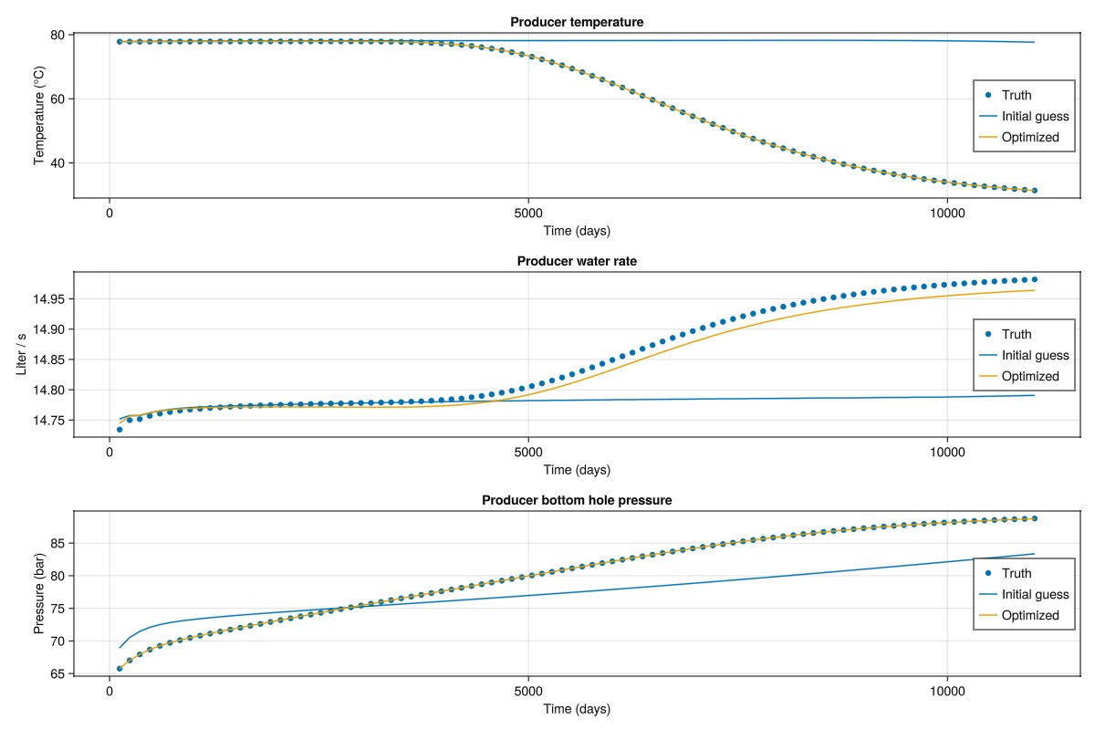

Plot the spatial results

We plot the spatial results for the truth case, the initial guess, and the optimized case. The temperature is plotted in Celsius and we use the same color scale for all steps. Note that in terms of the optimizer itself, this is hidden data: The objective function only matches the well responses. Getting a good match in the spatial distribution of temperature is a side-effect of the physics and parametrization of the model, as different physics or a different parameterization could lead to good match in terms of the objective function, even without good match for the spatial distribution.

step = 80
cmap = reverse(to_colormap(:heat))
fig = Figure(size = (1200, 400))
ax = Axis3(fig[1, 1], title = "Truth")
plot_cell_data!(ax, rmesh, states[step][:Temperature] .- 273.15, colorrange = (10.0, 100.0), colormap = cmap)
ax.elevation[] = 0.0
ax.azimuth[] = -π/2
hidedecorations!(ax)

ax = Axis3(fig[1, 2], title = "Initial guess")
plot_cell_data!(ax, rmesh, states_guess[step][:Temperature] .- 273.15, colorrange = (10.0, 100.0), colormap = cmap)
ax.elevation[] = 0.0
ax.azimuth[] = -π/2
hidedecorations!(ax)

ax = Axis3(fig[1, 3], title = "Optimized")
plt = plot_cell_data!(ax, rmesh, states_opt[step][:Temperature] .- 273.15, colorrange = (10.0, 100.0), colormap = cmap)
ax.elevation[] = 0.0
ax.azimuth[] = -π/2
hidedecorations!(ax)
Colorbar(fig[2, 1:3], plt, vertical = false)
fig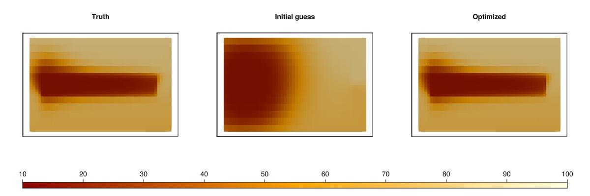

Set up control optimization

We can also use the same setup to perform control optimization, where we now can take advantage of the per-interval selection of rates and temperatures. Admittely, this problems is fairly simple, so the optimization is more conceptual than realistic: We define a new objective function that uses a fixed cost for the injected water (per degree times rate) and a similar value of produced heat. To make the optimization problem non-trivial, the cost of additional water (or higher temperature water) is significantly higher than the value of produced water with the same temperature.

temperature_injection_cost = 20.0
temperature_production_value = 8.0

function optimization_objective(m, s, dt, step_info, forces)
    T_at_prod = convert_from_si(compute_well_qoi(m, s, forces, :Producer, :temperature), :Celsius)
    T_at_inj = convert_from_si(forces[:Facility].control[:Injector].temperature, :Celsius)

    mass_rate_injector = compute_well_qoi(m, s, forces, :Injector, :mass_rate)
    mass_rate_producer = compute_well_qoi(m, s, forces, :Producer, :mass_rate)

    cost_inj = abs(mass_rate_injector) * T_at_inj * temperature_injection_cost
    value_prod = abs(mass_rate_producer) * T_at_prod * temperature_production_value
    return dt * (value_prod - cost_inj) / total_time
end

opt_ctrl = JutulDarcy.setup_reservoir_dict_optimization(prm_truth, setup_doublet_case)

DictParameters with 5 parameters (0 active), and 0 multipliers:
No active optimization parameters.
Inactive optimization parameters
┌─────────────────────────┬─────────────────────────────┬───────┬─────┬─────┐
│                    Name │ Initial value               │ Count │ Min │ Max │
├─────────────────────────┼─────────────────────────────┼───────┼─────┼─────┤
│     layer_heat_capacity │ 500.0, 600.0, 450.0         │     3 │   - │   - │
│          injection_rate │ 0.015 ± 3.47e-18            │    10 │   - │   - │
│ injection_temperature_C │ 15.0 ± 0.0                  │    10 │   - │   - │
│              layer_perm │ 9.87e-15, 7.9e-13, 1.97e-14 │     3 │   - │   - │
│        layer_porosities │ 0.1, 0.3, 0.1               │     3 │   - │   - │
└─────────────────────────┴─────────────────────────────┴───────┴─────┴─────┘
No multipliers set.

Set optimization to use injection rate and temperature

Note that as these are represented as per-interval values, we could also have passed vectors of equal length as the number of intervals for more fine-grained control over the limits. We specify that the dependencies include the whole case instead of just state0 and parameters since the forces depend on the optimization parameters.

free_optimization_parameter!(opt_ctrl, "injection_temperature_C", abs_max = 80.0, abs_min = 10.0)
free_optimization_parameter!(opt_ctrl, "injection_rate", abs_min = 1.0*liter/second, abs_max = 30.0*liter/second)

DictParameters with 5 parameters (2 active), and 0 multipliers:
Active optimization parameters
┌─────────────────────────┬──────────────────┬───────┬───────┬──────┐
│                    Name │ Initial value    │ Count │   Min │  Max │
├─────────────────────────┼──────────────────┼───────┼───────┼──────┤
│ injection_temperature_C │ 15.0 ± 0.0       │    10 │  10.0 │ 80.0 │
│          injection_rate │ 0.015 ± 3.47e-18 │    10 │ 0.001 │ 0.03 │
└─────────────────────────┴──────────────────┴───────┴───────┴──────┘
Inactive optimization parameters
┌─────────────────────┬─────────────────────────────┬───────┬─────┬─────┐
│                Name │ Initial value               │ Count │ Min │ Max │
├─────────────────────┼─────────────────────────────┼───────┼─────┼─────┤
│ layer_heat_capacity │ 500.0, 600.0, 450.0         │     3 │   - │   - │
│          layer_perm │ 9.87e-15, 7.9e-13, 1.97e-14 │     3 │   - │   - │
│    layer_porosities │ 0.1, 0.3, 0.1               │     3 │   - │   - │
└─────────────────────┴─────────────────────────────┴───────┴─────┴─────┘
No multipliers set.

Call the optimizer

prm_opt_ctrl = JutulDarcy.optimize_reservoir(opt_ctrl, optimization_objective, maximize = true, deps = :case, optimizer = :lbfgsb_qp);
opt_ctrl

DictParameters with 5 parameters (2 active), and 0 multipliers:
Active optimization parameters
┌─────────────────────────┬──────────────────┬───────┬───────┬──────┬───────────
│                    Name │ Initial value    │ Count │   Min │  Max │ Optimize ⋯
├─────────────────────────┼──────────────────┼───────┼───────┼──────┼───────────
│ injection_temperature_C │ 15.0 ± 0.0       │    10 │  10.0 │ 80.0 │ 14.5 ± 0 ⋯
│          injection_rate │ 0.015 ± 3.47e-18 │    10 │ 0.001 │ 0.03 │ 0.0116 ± ⋯
└─────────────────────────┴──────────────────┴───────┴───────┴──────┴───────────
                                                               2 columns omitted
Inactive optimization parameters
┌─────────────────────┬─────────────────────────────┬───────┬─────┬─────┐
│                Name │ Initial value               │ Count │ Min │ Max │
├─────────────────────┼─────────────────────────────┼───────┼─────┼─────┤
│ layer_heat_capacity │ 500.0, 600.0, 450.0         │     3 │   - │   - │
│          layer_perm │ 9.87e-15, 7.9e-13, 1.97e-14 │     3 │   - │   - │
│    layer_porosities │ 0.1, 0.3, 0.1               │     3 │   - │   - │
└─────────────────────┴─────────────────────────────┴───────┴─────┴─────┘
No multipliers set.

Plot the optimized injection rates and temperatures

The optimized injection rates and temperatures are plotted for each interval. The base case is shown in blue, while the optimized case is shown in orange. Note that the optimized case has reduced the injection temperature to the lower limit for all steps, and instead increase the injection rate significantly. The injection rate has a decrease part-way during the simulation, which increases the residence time of the injected water, allowing additional heat to be siphoned from the low permeable layers.

fig = Figure(size = (1200, 400))
ax = Axis(fig[1, 1], title = "Optimized injection temperature", ylabel = "Injection temperature (°C)", xlabel = "Interval")
scatter!(ax, prm_truth["injection_temperature_C"], label = "Base case")
scatter!(ax, prm_opt_ctrl["injection_temperature_C"], label = "Optimized case")
axislegend(position = :rc)

ax = Axis(fig[1, 2], title = "Optimized injection rate", ylabel = "Liter/second", xlabel = "Interval")
scatter!(ax, prm_truth["injection_rate"]./(liter/second), label = "Base case")
scatter!(ax, prm_opt_ctrl["injection_rate"]./(liter/second), label = "Optimized case")
axislegend(position = :rc)
fig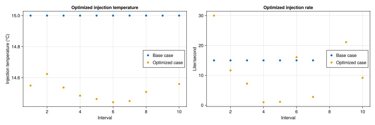

Simulate the optimized case

case_opt_ctrl = setup_doublet_case(prm_opt_ctrl)
ws_opt_ctrl, states_opt_ctrl = simulate_reservoir(case_opt_ctrl)

ReservoirSimResult with 92 entries:

  wells (2 present):
    :Producer
    :Injector
    Results per well:
       :lrat => Vector{Float64} of size (92,)
       :wrat => Vector{Float64} of size (92,)
       :temperature => Vector{Float64} of size (92,)
       :control => Vector{Symbol} of size (92,)
       :Aqueous_mass_rate => Vector{Float64} of size (92,)
       :bhp => Vector{Float64} of size (92,)
       :wcut => Vector{Float64} of size (92,)
       :mass_rate => Vector{Float64} of size (92,)
       :rate => Vector{Float64} of size (92,)
       :mrat => Vector{Float64} of size (92,)

  states (Vector with 92 entries, reservoir variables for each state)
    :Pressure => Vector{Float64} of size (1000,)
    :TotalMasses => Matrix{Float64} of size (1, 1000)
    :TotalThermalEnergy => Vector{Float64} of size (1000,)
    :FluidEnthalpy => Matrix{Float64} of size (1, 1000)
    :Temperature => Vector{Float64} of size (1000,)
    :PhaseMassDensities => Matrix{Float64} of size (1, 1000)
    :RockInternalEnergy => Vector{Float64} of size (1000,)
    :FluidInternalEnergy => Matrix{Float64} of size (1, 1000)

  time (report time for each state)
     Vector{Float64} of length 92

  result (extended states, reports)
     SimResult with 92 entries

  extra
     Dict{Any, Any} with keys :simulator, :config

  Completed at Jul. 02 2026 16:44 after 857 milliseconds, 303 microseconds, 71 nanoseconds.

Plot the distribution of temperature with and without optimization

step = 80
cmap = reverse(to_colormap(:heat))
fig = Figure(size = (1000, 400))
ax = Axis3(fig[1, 1], title = "Base case")
plot_cell_data!(ax, rmesh, states[step][:Temperature] .- 273.15, colorrange = (10.0, 100.0), colormap = cmap)
ax.elevation[] = 0.0
ax.azimuth[] = -π/2
hidedecorations!(ax)

ax = Axis3(fig[1, 2], title = "Optimized")
plt = plot_cell_data!(ax, rmesh, states_opt_ctrl[step][:Temperature] .- 273.15, colorrange = (10.0, 100.0), colormap = cmap)
ax.elevation[] = 0.0
ax.azimuth[] = -π/2
hidedecorations!(ax)
Colorbar(fig[2, 1:2], plt, vertical = false)
fig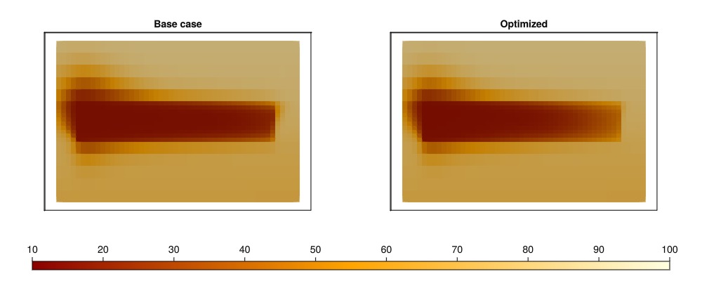

Plot the total thermal energy in the reservoir

The total thermal energy in the reservoir is computed as the sum of the thermal energy in each cell, which is the result of the rock heat capacity, porosity, fluid heat capacity and the temperature in each cell. The optimized strategy significantly decreases the remaining thermal energy in the reservoir, while still producing less cost than the base case according to our objective. The 2D nature of this problem makes it easy to recover a large amount energy, as the majority of the cells are swept by the cold front.

total_energy = map(s -> sum(s[:TotalThermalEnergy]), states)
total_energy_opt = map(s -> sum(s[:TotalThermalEnergy]), states_opt_ctrl)

fig = Figure(size = (1200, 400))
ax = Axis(fig[1, 1], title = "Total thermal energy", ylabel = "Total remaining energy (megajoules)", xlabel = "Time (days)")
t = ws.time ./ si_unit(:day)
lines!(ax, t, total_energy./1e6, label = "Base case")
lines!(ax, t, total_energy_opt./1e6, label = "Optimized case")
axislegend(position = :rc)
fig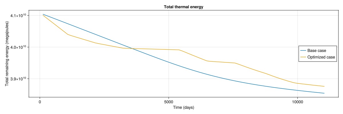

Example on GitHub

If you would like to run this example yourself, it can be downloaded from the JutulDarcy.jl GitHub repository as a script

This example took 371.882640441 seconds to complete.

---

This page was generated using Literate.jl.