Quarter-five-spot example

Immiscible   Introduction  

The quarter-five-spot is a standard test problem that simulates 1/4 of the five spot well pattern by assuming axial symmetry. The problem contains an injector in one corner and the producer in the opposing corner, with a significant volume of fluids injected into the domain.

using JutulDarcy, Jutul, HYPRE, Statistics
nx = 50;

Setup

We define a function that, for a given porosity field, computes a solution with an estimated permeability field. For assumptions and derivation of the specific form of the Kozeny-Carman relation used in this example, see Lie, Knut-Andreas. An introduction to reservoir simulation using MATLAB/GNU Octave: User guide for the MATLAB Reservoir Simulation Toolbox (MRST). Cambridge University Press, 2019, Section 2.5.2

function perm_kozeny_carman(Φ)
    return ((Φ^3)*(1e-5)^2)/(0.81*72*(1-Φ)^2);
end

function simulate_qfs(porosity = 0.3)
    Dx = 1000.0
    Dz = 10.0
    bar, kg, meter, day = si_units(:bar, :kilogram, :meter, :day)

    mesh = CartesianMesh((nx, nx, 1), (Dx, Dx, Dz))
    K = perm_kozeny_carman.(porosity)
    domain = reservoir_domain(mesh, permeability = K, porosity = porosity)
    Inj = setup_vertical_well(domain, 1, 1, name = :Injector);
    Prod = setup_vertical_well(domain, nx, nx, name = :Producer);
    phases = (LiquidPhase(), VaporPhase())
    rhoLS = 1000.0*kg/meter^3
    rhoGS = 700.0*kg/meter^3
    rhoS = [rhoLS, rhoGS]
    sys = ImmiscibleSystem(phases, reference_densities = rhoS)
    model, parameters = setup_reservoir_model(domain, sys, wells = [Inj, Prod])
    c = [1e-6/bar, 1e-6/bar]
    ρ = ConstantCompressibilityDensities(p_ref = 150*bar, density_ref = rhoS, compressibility = c)
    kr = BrooksCoreyRelativePermeabilities(sys, [2.0, 2.0])
    replace_variables!(model, PhaseMassDensities = ρ, RelativePermeabilities = kr);

    state0 = setup_reservoir_state(model, Pressure = 150*bar, Saturations = [1.0, 0.0])
    dt = repeat([30.0]*day, 12*10)
    dt = vcat([0.1, 1.0, 10.0], dt)
    inj_rate = Dx*Dx*Dz*0.3/sum(dt) # 1 PVI if average porosity is 0.3

    rate_target = TotalRateTarget(inj_rate)
    I_ctrl = InjectorControl(rate_target, [0.0, 1.0], density = rhoGS)
    bhp_target = BottomHolePressureTarget(50*bar)
    P_ctrl = ProducerControl(bhp_target)
    controls = Dict()
    controls[:Injector] = I_ctrl
    controls[:Producer] = P_ctrl
    forces = setup_reservoir_forces(model, control = controls)
    return simulate_reservoir(state0, model, dt, parameters = parameters, forces = forces, info_level = -1)
end

simulate_qfs (generic function with 2 methods)

Simulate base case

This will give the solution with uniform porosity of 0.3.

ws, states, report_time = simulate_qfs();

Plot the solution of the base case

We observe a radial flow pattern initially, before coning occurs near the producer well once the fluid has reached the opposite corner. The uniform permeability and porosity gives axial symmetry at $x=y$.

using GLMakie
to_2d(x) = reshape(vec(x), nx, nx)
get_sat(state) = to_2d(state[:Saturations][2, :])
nt = length(report_time)
fig = Figure()
h = nothing
ax = Axis(fig[1, 1])
h = contourf!(ax, get_sat(states[nt÷3]))
ax = Axis(fig[1, 2])
h = contourf!(ax, get_sat(states[nt]))
Colorbar(fig[1, end+1], h)
fig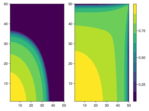

Create 10 realizations

We create a small set of realizations of the same model, with porosity that is uniformly varying between 0.1 and 0.3. The main idea is to get significantly different flow patterns as the porosity and permeability changes, and we will return to more realistic porosity fields later in this example.

function simulate_porosities(porosities)
    wellsols = []
    s = []
    report_step = Int(ceil(0.5*nt))
    for poro in porosities
        ws_i, states_i, rt = simulate_qfs(poro)
        push!(wellsols, ws_i)
        push!(s, get_sat(states_i[report_step]))
    end
    return (wellsols, s)
end
N = 10
porosities_uniform = []
for i in 1:N
    push!(porosities_uniform, 0.1 .+ 0.2*rand(Float64, (nx*nx)))
end
wells, saturations = simulate_porosities(porosities_uniform);

Plot the gas rate at the producer over the ensemble

using Statistics
function plot_wells(wellsols)
    fig = Figure(size = (1000, 600))
    ax = Axis(
        fig[1, 1],
        xlabel = "Time [days]",
        ylabel = "Gas rate [m³/s]",
        title = "Producer gas rate",
    )
    t = wellsols[1].time./si_units(:day)
    avg_rate = zeros(length(t))
    for ws in wellsols
        q = abs.(ws[:Producer][:grat])
        avg_rate += q
        lines!(ax, t, q, color = :grey)
    end
    avg_rate ./= length(wellsols)
    lines!(ax, t, avg_rate, color = :red, linewidth = 3, label = "Mean")
    axislegend(ax, position = :lt)
    xlims!(ax, [0.5mean(t), t[end]])
    fig
end

plot_wells(wells)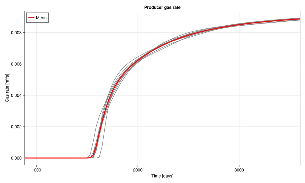

Plot the average saturation over the ensemble

avg = mean(saturations)
fig = Figure()
h = nothing
ax = Axis(fig[1, 1])
h = heatmap!(ax, avg, colorrange = (0.0, 1.0))
fig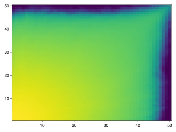

Plot a few realizations of porosity and resulting gas saturation

Note that the porosity fields are uniformly random without any spatial correlation.

function plot_realizations(sat, poro)
    fig = Figure(size = (1000, 400))
    poro_crange = (0.15, 0.25)
    sat_crange = (0.5, 1.0)
    h1 = h2 = nothing
    n_to_plot = 5
    for i in 1:n_to_plot
        ax = Axis(fig[1, i], title = "Gas saturation realization $i")
        h1 = heatmap!(ax, sat[i], colorrange = sat_crange)
        ax_poro = Axis(fig[2, i], title = "Porosity realization $i")
        h2 = heatmap!(ax_poro, to_2d(poro[i]), colorrange = poro_crange)
    end
    Colorbar(fig[1, n_to_plot+1], h1)
    Colorbar(fig[2, n_to_plot+1], h2)
    return fig
end
plot_realizations(saturations, porosities_uniform)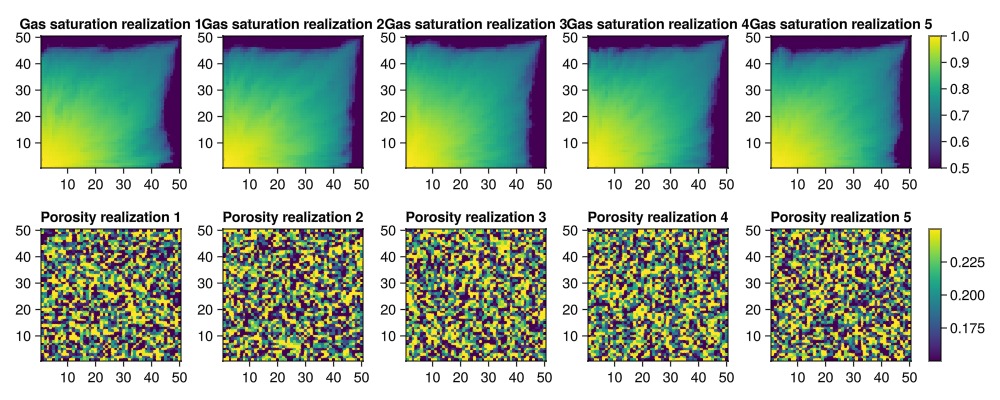

Use GeoStats.jl for more realistic porosity fields

Taking uniformly random samples is not a very realistic way to generate porosity fields. A more realistic approach is to use geostatistical methods from GeoStats.jl.

We here use a Gaussian process with a spherical covariance to generate the porosity fields. The setup is taken from the GeoStats.jl documentation which has more details on the approach.

import GeoStats: CartesianGrid, GaussianProcess, GaussianVariogram, SphericalCovariance, viz!
N = 30
grid = CartesianGrid(nx, nx)
proc = GaussianProcess(SphericalCovariance(range=30.0), 0.0)
real = rand(proc, grid, N)

2D Ensemble
  domain:    50×50 CartesianGrid
  variables: field
  N° reals:  30

Plot mean and variance of the realizations

m, v = mean(real), var(real)
fig = Figure(size = (800, 400))
axl = Axis(fig[1, 1], title = "Mean")
axr = Axis(fig[1, 2], title = "Variance")
viz!(axl, m.geometry, color = m.field)
viz!(axr, v.geometry, color = v.field)
fig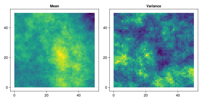

Run simulations with the new porosity fields

We here map the realizations to porosity values between 0.05 and 0.195, and run the simulations. Note that in a more realistic workflow we would condition the process on data instead of taking unconditional realizations.

to_poro(x) = 0.2 + 0.1*clamp(x, -2.0, 2.0)/4.0
porosities_gaussian = map(i -> to_poro.(real[i].field), 1:N)
wells_gaussian, saturations_gaussian = simulate_porosities(porosities_gaussian);

Plot the producer rate over the ensemble

plot_wells(wells_gaussian)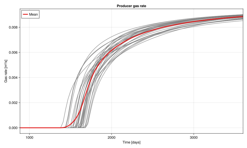

Plot a few realizations for the Gaussian porosity fields

We observe that the porosity fields now have spatial correlation.

plot_realizations(saturations_gaussian, porosities_gaussian)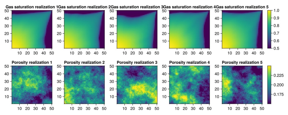

Example on GitHub

If you would like to run this example yourself, it can be downloaded from the JutulDarcy.jl GitHub repository as a script, or as a Jupyter Notebook

This example took 160.406525145 seconds to complete.

---

This page was generated using Literate.jl.