High-temperature Aquifer Thermal Energy Storage (HT-ATES)

This example demonstrates how to simulate high-temperature aquifer thermal energy storage. We set up a simple case describing a vertical slice of a reservoir with an a main (hot) well near the left boundary, and a supporting (cold) well near the right boundary. The reservoir has boundarys condition that provides a constant pressure and temperature. We set up a yearly cycle where energy is stored from June to September, and discharged from December to March. The rest of the year is a rest period where no energy is stored or produced.

using JutulDarcy, Jutul, HYPRE
import Dates: monthname
darcy, litre, year, second = si_units(:darcy, :litre, :year, :second)

nx = 100
nz = 100

temperature_top = convert_to_si(40.0, :Celsius)
pressure_top = convert_to_si(120.0, :bar)
temperature_surface = convert_to_si(10.0, :Celsius)

grad_p = 1000*9.81
grad_T = 0.3

0.3

Set up the reservoir

g = CartesianMesh((nx, 1, nz), (250.0, 250.0, 75.0))
reservoir = reservoir_domain(g,
    permeability = [0.3, 0.3, 0.1].*darcy,
    porosity = 0.3,
    rock_thermal_conductivity = 2.0,
    fluid_thermal_conductivity = 0.6
)

depth = reservoir[:cell_centroids][3, :];

Define wells and model

di = Int(ceil(nx/4))
k = Int(ceil(nz/2))
Whot = setup_vertical_well(reservoir, 0+di   , 1, toe = k, name = :Hot)
Wcold = setup_vertical_well(reservoir, nx-di+1, 1, toe = k, name = :Cold)

model, parameters = setup_reservoir_model(reservoir, :geothermal, wells = [Whot, Wcold]);

Set up boundary and initial conditions

bcells = Int[]
pressure_res = Float64[]
temperature_res = Float64[]
for cell in 1:number_of_cells(g)
    d = depth[cell]
    push!(pressure_res, pressure_top + grad_p*d)
    push!(temperature_res, temperature_top + grad_T*d)

    I, J, K = cell_ijk(g, cell)
    if I == 1 || I == nx
        push!(bcells, cell)
    end
end

bc = flow_boundary_condition(bcells, reservoir, pressure_res[bcells], temperature_res[bcells]);

Set up the schedule

Set up forces

We assume we have a supply amounting to 90°C. at 25 l/s for storage. During the discharge period, we assume the same discharge rate and a temperature of 10°C.

charge_rate = 25litre/second
discharge_rate = charge_rate
temperature_charge = temperature_top + 50.0
temperature_discharge = temperature_top - 30.0

283.15

Set up forces for charging

rate_target = TotalRateTarget(charge_rate)
ctrl_hot  = InjectorControl(rate_target, [1.0], density = 1000.0, temperature = temperature_charge)
rate_target = TotalRateTarget(-charge_rate)
ctrl_cold = ProducerControl(rate_target)
forces_charge = setup_reservoir_forces(model, control = Dict(:Hot => ctrl_hot, :Cold => ctrl_cold), bc = bc)

Dict{Symbol, Any} with 4 entries:
  :Hot       => (mask = nothing,)
  :Cold      => (mask = nothing,)
  :Reservoir => (bc = FlowBoundaryCondition{Int64, Float64, Nothing}[FlowBounda…
  :Facility  => (control = Dict{Symbol, WellControlForce}(:Hot=>InjectorControl…

Set up forces for discharging

rate_target = TotalRateTarget(discharge_rate)
ctrl_cold = InjectorControl(rate_target, [1.0], density = 1000.0, temperature = temperature_discharge)
rate_target = TotalRateTarget(-discharge_rate)
ctrl_hot = ProducerControl(rate_target)
forces_discharge = setup_reservoir_forces(model, control = Dict(:Hot => ctrl_hot, :Cold => ctrl_cold), bc = bc)

Dict{Symbol, Any} with 4 entries:
  :Hot       => (mask = nothing,)
  :Cold      => (mask = nothing,)
  :Reservoir => (bc = FlowBoundaryCondition{Int64, Float64, Nothing}[FlowBounda…
  :Facility  => (control = Dict{Symbol, WellControlForce}(:Hot=>ProducerControl…

Set up forces for rest period

forces_rest = setup_reservoir_forces(model, bc = bc)

Dict{Symbol, Any} with 4 entries:
  :Hot       => (mask = nothing,)
  :Cold      => (mask = nothing,)
  :Reservoir => (bc = FlowBoundaryCondition{Int64, Float64, Nothing}[FlowBounda…
  :Facility  => (control = Dict{Symbol, Any}(:Hot=>DisabledControl{DisabledTarg…

Set up timesteps and assign forces to each timestep

num_years = 25
dt = Float64[]
forces = []
month = year/12
for year in 1:num_years
    for mno in vcat(6:12, 1:5)
        mname = monthname(mno)
        if mname in ("January", "February", "March", "December")
            push!(dt, month)
            push!(forces, forces_discharge)
        elseif mname in ("June", "July", "August", "September")
            push!(dt, month)
            push!(forces, forces_charge)
        else
            @assert mname in ("April", "May", "October", "November")
            push!(dt, month)
            push!(forces, forces_rest)
        end
    end
end

Set up initial state

state0 = setup_reservoir_state(model, Pressure = pressure_res, Temperature = temperature_res);

Simulate the case

ws, states = simulate_reservoir(state0, model, dt,
    forces = forces,
    parameters = parameters
);

Jutul: Simulating 25 years as 300 report steps
╭────────────────┬───────────┬───────────────┬──────────╮
│ Iteration type │  Avg/step │  Avg/ministep │    Total │
│                │ 300 steps │ 306 ministeps │ (wasted) │
├────────────────┼───────────┼───────────────┼──────────┤
│ Newton         │      3.57 │           3.5 │ 1071 (0) │
│ Linearization  │      4.59 │           4.5 │ 1377 (0) │
│ Linear solver  │   9.72333 │       9.53268 │ 2917 (0) │
│ Precond apply  │   19.4467 │       19.0654 │ 5834 (0) │
╰────────────────┴───────────┴───────────────┴──────────╯
╭───────────────┬─────────┬────────────┬─────────╮
│ Timing type   │    Each │   Relative │   Total │
│               │      ms │ Percentage │       s │
├───────────────┼─────────┼────────────┼─────────┤
│ Properties    │  0.9991 │     4.06 % │  1.0700 │
│ Equations     │  6.0389 │    31.57 % │  8.3155 │
│ Assembly      │  0.9033 │     4.72 % │  1.2438 │
│ Linear solve  │  1.0140 │     4.12 % │  1.0860 │
│ Linear setup  │  6.1216 │    24.89 % │  6.5562 │
│ Precond apply │  0.8342 │    18.47 % │  4.8665 │
│ Update        │  0.4043 │     1.64 % │  0.4331 │
│ Convergence   │  0.5693 │     2.98 % │  0.7840 │
│ Input/Output  │  0.4664 │     0.54 % │  0.1427 │
│ Other         │  1.7236 │     7.01 % │  1.8460 │
├───────────────┼─────────┼────────────┼─────────┤
│ Total         │ 24.5974 │   100.00 % │ 26.3438 │
╰───────────────┴─────────┴────────────┴─────────╯

Plot the reservoir states in the interactive viewer

using GLMakie
plot_reservoir(model, states, key = :Temperature, step = num_years*12)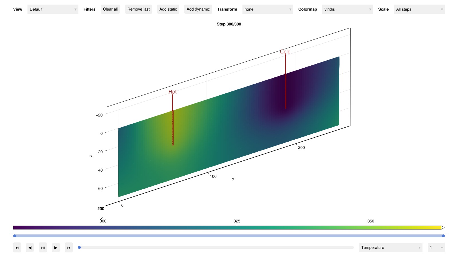

Plot wells interactively

plot_well_results(ws)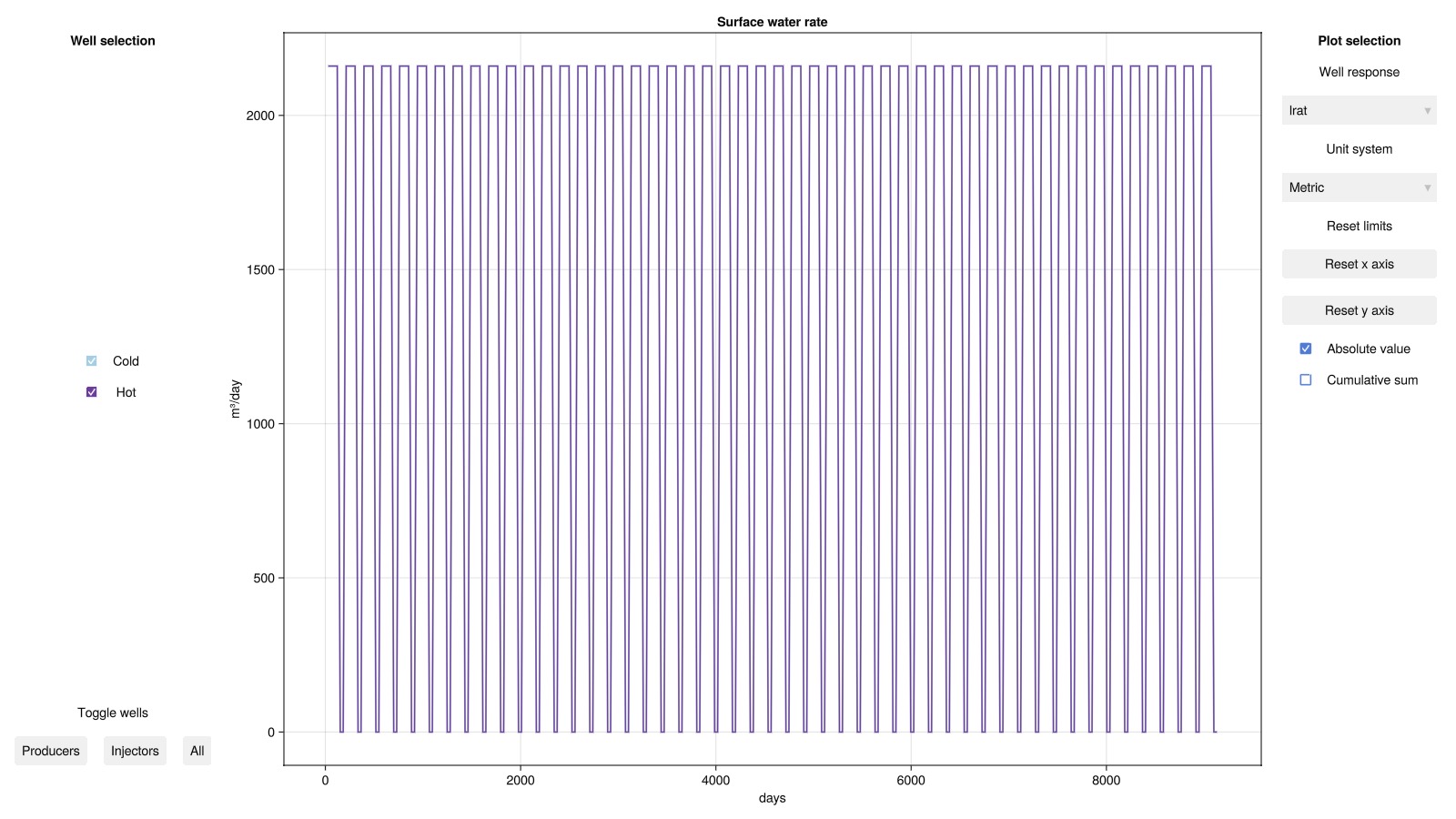

Plot energy recovery factor

The energy recovery factor η is defined as the amount of stored to produced energy. We plot this both cumulatively and for each of the 25 yearly cycles

wd = ws.wells[:Hot]
c_p_water = 4.186 # kJ/kgK

well_temp = wd[:temperature]
q = wd[:mass_rate]

storage = q .> 0
q_store = q.*storage
q_prod = q.*(.!storage)
stored_energy = well_temp.*q_store.*c_p_water.*dt
produced_energy = -well_temp.*q_prod.*c_p_water.*dt
η_cumulative = cumsum(produced_energy)./cumsum(stored_energy)
t = cumsum(dt)./si_unit(:day)

η, T = zeros(num_years), zeros(num_years)
for i = 1:num_years
    ix = (1:12) .+ 12*(i-1)
    se = sum(stored_energy[ix])
    pe = sum(produced_energy[ix])
    η[i] = pe/se
    T[i] = t[ix[end]]
end

fig = Figure()
ax = Axis(fig[1, 1], title = "Produced energy [kJ]")
barplot!(ax, T, η, label = "Yearly")
lines!(ax, t, η_cumulative, color = :black, label = "Cumulative")
axislegend(ax, position = :rb)
fig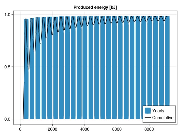

Example on GitHub

If you would like to run this example yourself, it can be downloaded from the JutulDarcy.jl GitHub repository as a script, or as a Jupyter Notebook

This example took 49.731295227 seconds to complete.

---

This page was generated using Literate.jl.