Compositional simulation with Clapeyron.jl equations of state

Compositional   Advanced  

This example shows how to set up and run a compositional simulation using equations of state from the Clapeyron.jl package.

The compositional solver in JutulDarcy uses the MultiComponentFlash.jl package for phase equilibrium calculations by defalt, but it is also possible to use other packages that implement the required interface. Here, we demonstrate how to use the JutulDarcy package extension for Clapeyron.jl to set up a compositional simulation using two different equations of state.

# Import packages and define helper function
using Jutul, JutulDarcy, GLMakie, MultiComponentFlash

function solve_and_plot_displacement(eos, nx = 50; name = "")
    g = CartesianMesh((nx, 1, 1), (100.0, 10.0, 10.0))
    Darcy, bar, kg, meter, day = si_units(:darcy, :bar, :kilogram, :meter, :day)
    res = reservoir_domain(g, porosity = 0.3, permeability = 0.1*Darcy)
    inj = setup_well(res, 1, name = :Injector)
    prod = setup_well(res, nx, name = :Producer)
    L, V = LiquidPhase(), VaporPhase()
    sys = MultiPhaseCompositionalSystemLV(eos, (L, V))
    model = setup_reservoir_model(res, sys, wells = [inj, prod], extra_out = false);
    state0 = setup_reservoir_state(model, Pressure = 50*bar, OverallMoleFractions = [0.0, 1.0]);
    dt = fill(30*day, 12)
    rate_target = TotalRateTarget(sum(pore_volume(res))/ sum(dt))
    I_ctrl = InjectorControl(rate_target, [1.0, 0.0], density = 100.0*kg/meter^3)
    bhp_target = BottomHolePressureTarget(50*bar)
    P_ctrl = ProducerControl(bhp_target)
    controls = Dict()
    controls[:Injector] = I_ctrl
    controls[:Producer] = P_ctrl
    forces = setup_reservoir_forces(model, control = controls)
    _, states = simulate_reservoir(state0, model, dt, forces = forces)

    state = states[end]
    sg = state[:Saturations][2, :]
    z1 = state[:OverallMoleFractions][1, :]
    z2 = state[:OverallMoleFractions][2, :]
    x_c = res[:cell_centroids][1, :]
    fig = Figure()
    ax = Axis(fig[1, 1], xlabel = "x [m]", title = name)
    lines!(ax, x_c, sg, label = "Gas saturation")
    cnames = MultiComponentFlash.component_names(eos)
    lines!(ax, x_c, z1, label = "C1: $(cnames[1]) mole fraction")
    lines!(ax, x_c, z2, label = "C2: $(cnames[2]) mole fraction")
    axislegend(position = :rc)
    fig
end

solve_and_plot_displacement (generic function with 2 methods)

Define components and mixture

We here define a binary mixture of methane and carbon dioxide and 50 grid cells for simulation.

nx = 50
components = ["carbondioxide", "decane"]

2-element Vector{String}:
 "carbondioxide"
 "decane"

Simulate Peng-Robinson EOS

import Clapeyron: PR
solve_and_plot_displacement(PR(components), nx, name = "Peng-Robinson (PR, Clapeyron) EOS")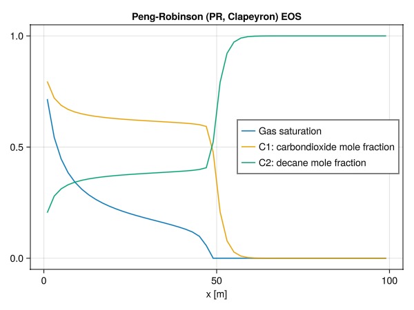

Simulate Soave-Redlich-Kwong EOS

We can easily switch to another equation of state, e.g., the Soave-Redlich-Kwong EOS. Note that the displacement front is a bit different relative to the Peng-Robinson EOS, which is expected since we have used the EOS without adjusting any parameters for the mixtures.

import Clapeyron: SRK
solve_and_plot_displacement(SRK(components), nx, name = "Soave-Redlich-Kwong (SRK, Clapeyron.jl) EOS")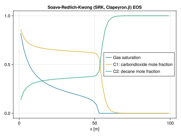

Conclusion

We see that it is possible to use equations of state from Clapeyron.jl in JutulDarcy to run compositional simulations. The Clapeyron.jl package provides a wide range of equations-of-state that significantly extends the capabilities of the compositional solver.

Note that the default flash used in the compositional solver in JutulDarcy is quite tailored towards coupling with a simulator, both in terms of complexity and code structure. For this reason, other implementations of equations of state may be slower in practice. It is recommended that you test the performance of your chosen equation of state on a test problem like we did here before setting up a large simulation.

Example on GitHub

If you would like to run this example yourself, it can be downloaded from the JutulDarcy.jl GitHub repository as a script, or as a Jupyter Notebook

This example took 171.577626941 seconds to complete.

---

This page was generated using Literate.jl.