Model coarsening
Running a model at full resolution can be computationally expensive. In many cases, it is possible to coarsen the model to reduce the computational cost. This example demonstrates how to coarsen a model using JutulDarcy.jl. The example uses the Egg model, which is a small oil-water model with heterogeneous permeability. The model is coarsened using different methods and partition sizes, and the results are compared to the fine-scale model. The example demonstrates how to coarsen a model and simulate it using JutulDarcy.jl. The example also demonstrates how to compare the results of the coarse-scale model to the fine-scale model.
The example is intended to show the workflow of coarsening a model, and represents a starting point for more advanced techniques like upscaling, coarse-model calibration and history matching. The model is therefore intentionally simple and very coarse for quick simulations, and not necessarily accurate model responses.
using Jutul, JutulDarcy, HYPRE
using GLMakie
using GeoEnergyIO
data_dir = GeoEnergyIO.test_input_file_path("EGG")
data_pth = joinpath(data_dir, "EGG.DATA")
fine_case = setup_case_from_data_file(data_pth);
Simulate the base case
We simulate the fine case to get a reference solution to compare against. We also extract the mesh and reservoir for plotting.
fine_model = fine_case.model
fine_reservoir = reservoir_domain(fine_model)
fine_mesh = physical_representation(fine_reservoir)
ws, states = simulate_reservoir(fine_case, info_level = 1);[92;1mJutul:[0m Simulating 9 years, 44.69 weeks as 135 report steps
[34;1mStep 1/135:[0m Solving start to 1 day, Δt = 1 day
[34;1mStep 2/135:[0m Solving 1 day to 5 days, Δt = 4 days
[34;1mStep 3/135:[0m Solving 5 days to 1 week, 3 days, Δt = 5 days
[34;1mStep 4/135:[0m Solving 1 week, 3 days to 2 weeks, 6 days, Δt = 1 week, 3 days
[34;1mStep 5/135:[0m Solving 2 weeks, 6 days to 4 weeks, 2 days, Δt = 1 week, 3 days
[34;1mStep 6/135:[0m Solving 4 weeks, 2 days to 5 weeks, 5 days, Δt = 1 week, 3 days
[34;1mStep 7/135:[0m Solving 5 weeks, 5 days to 7 weeks, 1 day, Δt = 1 week, 3 days
[34;1mStep 8/135:[0m Solving 7 weeks, 1 day to 8 weeks, 4 days, Δt = 1 week, 3 days
[34;1mStep 9/135:[0m Solving 8 weeks, 4 days to 10 weeks, Δt = 1 week, 3 days
[34;1mStep 10/135:[0m Solving 10 weeks to 11 weeks, 3 days, Δt = 1 week, 3 days
[34;1mStep 11/135:[0m Solving 11 weeks, 3 days to 12 weeks, 6 days, Δt = 1 week, 3 days
[34;1mStep 12/135:[0m Solving 12 weeks, 6 days to 15 weeks, Δt = 2 weeks, 1 day
[34;1mStep 13/135:[0m Solving 15 weeks to 17 weeks, 1 day, Δt = 2 weeks, 1 day
[34;1mStep 14/135:[0m Solving 17 weeks, 1 day to 19 weeks, 2 days, Δt = 2 weeks, 1 day
[34;1mStep 15/135:[0m Solving 19 weeks, 2 days to 21 weeks, 3 days, Δt = 2 weeks, 1 day
[34;1mStep 16/135:[0m Solving 21 weeks, 3 days to 23 weeks, 4 days, Δt = 2 weeks, 1 day
[34;1mStep 17/135:[0m Solving 23 weeks, 4 days to 25 weeks, 5 days, Δt = 2 weeks, 1 day
[34;1mStep 18/135:[0m Solving 25 weeks, 5 days to 27 weeks, 6 days, Δt = 2 weeks, 1 day
[34;1mStep 19/135:[0m Solving 27 weeks, 6 days to 30 weeks, Δt = 2 weeks, 1 day
[34;1mStep 20/135:[0m Solving 30 weeks to 32 weeks, 1 day, Δt = 2 weeks, 1 day
[34;1mStep 21/135:[0m Solving 32 weeks, 1 day to 34 weeks, 2 days, Δt = 2 weeks, 1 day
[34;1mStep 22/135:[0m Solving 34 weeks, 2 days to 36 weeks, 3 days, Δt = 2 weeks, 1 day
[34;1mStep 23/135:[0m Solving 36 weeks, 3 days to 38 weeks, 4 days, Δt = 2 weeks, 1 day
[34;1mStep 24/135:[0m Solving 38 weeks, 4 days to 40 weeks, 5 days, Δt = 2 weeks, 1 day
[34;1mStep 25/135:[0m Solving 40 weeks, 5 days to 42 weeks, 6 days, Δt = 2 weeks, 1 day
[34;1mStep 26/135:[0m Solving 42 weeks, 6 days to 47 weeks, 1 day, Δt = 4 weeks, 2 days
[34;1mStep 27/135:[0m Solving 47 weeks, 1 day to 51 weeks, 3 days, Δt = 4 weeks, 2 days
[34;1mStep 28/135:[0m Solving 51 weeks, 3 days to 1 year, 3.537 weeks, Δt = 4 weeks, 2 days
[34;1mStep 29/135:[0m Solving 1 year, 3.537 weeks to 1 year, 7.822 weeks, Δt = 4 weeks, 2 days
[34;1mStep 30/135:[0m Solving 1 year, 7.822 weeks to 1 year, 12.11 weeks, Δt = 4 weeks, 2 days
[34;1mStep 31/135:[0m Solving 1 year, 12.11 weeks to 1 year, 16.39 weeks, Δt = 4 weeks, 2 days
[34;1mStep 32/135:[0m Solving 1 year, 16.39 weeks to 1 year, 20.68 weeks, Δt = 4 weeks, 2 days
[34;1mStep 33/135:[0m Solving 1 year, 20.68 weeks to 1 year, 24.97 weeks, Δt = 4 weeks, 2 days
[34;1mStep 34/135:[0m Solving 1 year, 24.97 weeks to 1 year, 29.25 weeks, Δt = 4 weeks, 2 days
[34;1mStep 35/135:[0m Solving 1 year, 29.25 weeks to 1 year, 33.54 weeks, Δt = 4 weeks, 2 days
[34;1mStep 36/135:[0m Solving 1 year, 33.54 weeks to 1 year, 37.82 weeks, Δt = 4 weeks, 2 days
[34;1mStep 37/135:[0m Solving 1 year, 37.82 weeks to 1 year, 42.11 weeks, Δt = 4 weeks, 2 days
[34;1mStep 38/135:[0m Solving 1 year, 42.11 weeks to 1 year, 46.39 weeks, Δt = 4 weeks, 2 days
[34;1mStep 39/135:[0m Solving 1 year, 46.39 weeks to 1 year, 50.68 weeks, Δt = 4 weeks, 2 days
[34;1mStep 40/135:[0m Solving 1 year, 50.68 weeks to 2 years, 2.788 weeks, Δt = 4 weeks, 2 days
[34;1mStep 41/135:[0m Solving 2 years, 2.788 weeks to 2 years, 7.074 weeks, Δt = 4 weeks, 2 days
[34;1mStep 42/135:[0m Solving 2 years, 7.074 weeks to 2 years, 11.36 weeks, Δt = 4 weeks, 2 days
[34;1mStep 43/135:[0m Solving 2 years, 11.36 weeks to 2 years, 15.64 weeks, Δt = 4 weeks, 2 days
[34;1mStep 44/135:[0m Solving 2 years, 15.64 weeks to 2 years, 19.93 weeks, Δt = 4 weeks, 2 days
[34;1mStep 45/135:[0m Solving 2 years, 19.93 weeks to 2 years, 24.22 weeks, Δt = 4 weeks, 2 days
[34;1mStep 46/135:[0m Solving 2 years, 24.22 weeks to 2 years, 28.5 weeks, Δt = 4 weeks, 2 days
[34;1mStep 47/135:[0m Solving 2 years, 28.5 weeks to 2 years, 32.79 weeks, Δt = 4 weeks, 2 days
[34;1mStep 48/135:[0m Solving 2 years, 32.79 weeks to 2 years, 37.07 weeks, Δt = 4 weeks, 2 days
[34;1mStep 49/135:[0m Solving 2 years, 37.07 weeks to 2 years, 41.36 weeks, Δt = 4 weeks, 2 days
[34;1mStep 50/135:[0m Solving 2 years, 41.36 weeks to 2 years, 45.65 weeks, Δt = 4 weeks, 2 days
[34;1mStep 51/135:[0m Solving 2 years, 45.65 weeks to 2 years, 49.93 weeks, Δt = 4 weeks, 2 days
[34;1mStep 52/135:[0m Solving 2 years, 49.93 weeks to 3 years, 2.039 weeks, Δt = 4 weeks, 2 days
[34;1mStep 53/135:[0m Solving 3 years, 2.039 weeks to 3 years, 6.325 weeks, Δt = 4 weeks, 2 days
[34;1mStep 54/135:[0m Solving 3 years, 6.325 weeks to 3 years, 10.61 weeks, Δt = 4 weeks, 2 days
[34;1mStep 55/135:[0m Solving 3 years, 10.61 weeks to 3 years, 14.9 weeks, Δt = 4 weeks, 2 days
[34;1mStep 56/135:[0m Solving 3 years, 14.9 weeks to 3 years, 19.18 weeks, Δt = 4 weeks, 2 days
[34;1mStep 57/135:[0m Solving 3 years, 19.18 weeks to 3 years, 23.47 weeks, Δt = 4 weeks, 2 days
[34;1mStep 58/135:[0m Solving 3 years, 23.47 weeks to 3 years, 27.75 weeks, Δt = 4 weeks, 2 days
[34;1mStep 59/135:[0m Solving 3 years, 27.75 weeks to 3 years, 32.04 weeks, Δt = 4 weeks, 2 days
[34;1mStep 60/135:[0m Solving 3 years, 32.04 weeks to 3 years, 36.32 weeks, Δt = 4 weeks, 2 days
[34;1mStep 61/135:[0m Solving 3 years, 36.32 weeks to 3 years, 40.61 weeks, Δt = 4 weeks, 2 days
[34;1mStep 62/135:[0m Solving 3 years, 40.61 weeks to 3 years, 44.9 weeks, Δt = 4 weeks, 2 days
[34;1mStep 63/135:[0m Solving 3 years, 44.9 weeks to 3 years, 49.18 weeks, Δt = 4 weeks, 2 days
[34;1mStep 64/135:[0m Solving 3 years, 49.18 weeks to 4 years, 1.29 week, Δt = 4 weeks, 2 days
[34;1mStep 65/135:[0m Solving 4 years, 1.29 week to 4 years, 5.576 weeks, Δt = 4 weeks, 2 days
[34;1mStep 66/135:[0m Solving 4 years, 5.576 weeks to 4 years, 9.861 weeks, Δt = 4 weeks, 2 days
[34;1mStep 67/135:[0m Solving 4 years, 9.861 weeks to 4 years, 14.15 weeks, Δt = 4 weeks, 2 days
[34;1mStep 68/135:[0m Solving 4 years, 14.15 weeks to 4 years, 18.43 weeks, Δt = 4 weeks, 2 days
[34;1mStep 69/135:[0m Solving 4 years, 18.43 weeks to 4 years, 22.72 weeks, Δt = 4 weeks, 2 days
[34;1mStep 70/135:[0m Solving 4 years, 22.72 weeks to 4 years, 27 weeks, Δt = 4 weeks, 2 days
[34;1mStep 71/135:[0m Solving 4 years, 27 weeks to 4 years, 31.29 weeks, Δt = 4 weeks, 2 days
[34;1mStep 72/135:[0m Solving 4 years, 31.29 weeks to 4 years, 35.58 weeks, Δt = 4 weeks, 2 days
[34;1mStep 73/135:[0m Solving 4 years, 35.58 weeks to 4 years, 39.86 weeks, Δt = 4 weeks, 2 days
[34;1mStep 74/135:[0m Solving 4 years, 39.86 weeks to 4 years, 44.15 weeks, Δt = 4 weeks, 2 days
[34;1mStep 75/135:[0m Solving 4 years, 44.15 weeks to 4 years, 48.43 weeks, Δt = 4 weeks, 2 days
[34;1mStep 76/135:[0m Solving 4 years, 48.43 weeks to 5 years, 3.788 days, Δt = 4 weeks, 2 days
[34;1mStep 77/135:[0m Solving 5 years, 3.788 days to 5 years, 4.827 weeks, Δt = 4 weeks, 2 days
[34;1mStep 78/135:[0m Solving 5 years, 4.827 weeks to 5 years, 9.113 weeks, Δt = 4 weeks, 2 days
[34;1mStep 79/135:[0m Solving 5 years, 9.113 weeks to 5 years, 13.4 weeks, Δt = 4 weeks, 2 days
[34;1mStep 80/135:[0m Solving 5 years, 13.4 weeks to 5 years, 17.68 weeks, Δt = 4 weeks, 2 days
[34;1mStep 81/135:[0m Solving 5 years, 17.68 weeks to 5 years, 21.97 weeks, Δt = 4 weeks, 2 days
[34;1mStep 82/135:[0m Solving 5 years, 21.97 weeks to 5 years, 26.26 weeks, Δt = 4 weeks, 2 days
[34;1mStep 83/135:[0m Solving 5 years, 26.26 weeks to 5 years, 30.54 weeks, Δt = 4 weeks, 2 days
[34;1mStep 84/135:[0m Solving 5 years, 30.54 weeks to 5 years, 34.83 weeks, Δt = 4 weeks, 2 days
[34;1mStep 85/135:[0m Solving 5 years, 34.83 weeks to 5 years, 39.11 weeks, Δt = 4 weeks, 2 days
[34;1mStep 86/135:[0m Solving 5 years, 39.11 weeks to 5 years, 43.4 weeks, Δt = 4 weeks, 2 days
[34;1mStep 87/135:[0m Solving 5 years, 43.4 weeks to 5 years, 47.68 weeks, Δt = 4 weeks, 2 days
[34;1mStep 88/135:[0m Solving 5 years, 47.68 weeks to 5 years, 51.97 weeks, Δt = 4 weeks, 2 days
[34;1mStep 89/135:[0m Solving 5 years, 51.97 weeks to 6 years, 4.078 weeks, Δt = 4 weeks, 2 days
[34;1mStep 90/135:[0m Solving 6 years, 4.078 weeks to 6 years, 8.364 weeks, Δt = 4 weeks, 2 days
[34;1mStep 91/135:[0m Solving 6 years, 8.364 weeks to 6 years, 12.65 weeks, Δt = 4 weeks, 2 days
[34;1mStep 92/135:[0m Solving 6 years, 12.65 weeks to 6 years, 16.93 weeks, Δt = 4 weeks, 2 days
[34;1mStep 93/135:[0m Solving 6 years, 16.93 weeks to 6 years, 21.22 weeks, Δt = 4 weeks, 2 days
[34;1mStep 94/135:[0m Solving 6 years, 21.22 weeks to 6 years, 25.51 weeks, Δt = 4 weeks, 2 days
[34;1mStep 95/135:[0m Solving 6 years, 25.51 weeks to 6 years, 29.79 weeks, Δt = 4 weeks, 2 days
[34;1mStep 96/135:[0m Solving 6 years, 29.79 weeks to 6 years, 34.08 weeks, Δt = 4 weeks, 2 days
[34;1mStep 97/135:[0m Solving 6 years, 34.08 weeks to 6 years, 38.36 weeks, Δt = 4 weeks, 2 days
[34;1mStep 98/135:[0m Solving 6 years, 38.36 weeks to 6 years, 42.65 weeks, Δt = 4 weeks, 2 days
[34;1mStep 99/135:[0m Solving 6 years, 42.65 weeks to 6 years, 46.94 weeks, Δt = 4 weeks, 2 days
[34;1mStep 100/135:[0m Solving 6 years, 46.94 weeks to 6 years, 51.22 weeks, Δt = 4 weeks, 2 days
[34;1mStep 101/135:[0m Solving 6 years, 51.22 weeks to 7 years, 3.329 weeks, Δt = 4 weeks, 2 days
[34;1mStep 102/135:[0m Solving 7 years, 3.329 weeks to 7 years, 7.615 weeks, Δt = 4 weeks, 2 days
[34;1mStep 103/135:[0m Solving 7 years, 7.615 weeks to 7 years, 11.9 weeks, Δt = 4 weeks, 2 days
[34;1mStep 104/135:[0m Solving 7 years, 11.9 weeks to 7 years, 16.19 weeks, Δt = 4 weeks, 2 days
[34;1mStep 105/135:[0m Solving 7 years, 16.19 weeks to 7 years, 20.47 weeks, Δt = 4 weeks, 2 days
[34;1mStep 106/135:[0m Solving 7 years, 20.47 weeks to 7 years, 24.76 weeks, Δt = 4 weeks, 2 days
[34;1mStep 107/135:[0m Solving 7 years, 24.76 weeks to 7 years, 29.04 weeks, Δt = 4 weeks, 2 days
[34;1mStep 108/135:[0m Solving 7 years, 29.04 weeks to 7 years, 33.33 weeks, Δt = 4 weeks, 2 days
[34;1mStep 109/135:[0m Solving 7 years, 33.33 weeks to 7 years, 37.61 weeks, Δt = 4 weeks, 2 days
[34;1mStep 110/135:[0m Solving 7 years, 37.61 weeks to 7 years, 41.9 weeks, Δt = 4 weeks, 2 days
[34;1mStep 111/135:[0m Solving 7 years, 41.9 weeks to 7 years, 46.19 weeks, Δt = 4 weeks, 2 days
[34;1mStep 112/135:[0m Solving 7 years, 46.19 weeks to 7 years, 50.47 weeks, Δt = 4 weeks, 2 days
[34;1mStep 113/135:[0m Solving 7 years, 50.47 weeks to 8 years, 2.58 weeks, Δt = 4 weeks, 2 days
[34;1mStep 114/135:[0m Solving 8 years, 2.58 weeks to 8 years, 6.866 weeks, Δt = 4 weeks, 2 days
[34;1mStep 115/135:[0m Solving 8 years, 6.866 weeks to 8 years, 11.15 weeks, Δt = 4 weeks, 2 days
[34;1mStep 116/135:[0m Solving 8 years, 11.15 weeks to 8 years, 15.44 weeks, Δt = 4 weeks, 2 days
[34;1mStep 117/135:[0m Solving 8 years, 15.44 weeks to 8 years, 19.72 weeks, Δt = 4 weeks, 2 days
[34;1mStep 118/135:[0m Solving 8 years, 19.72 weeks to 8 years, 24.01 weeks, Δt = 4 weeks, 2 days
[34;1mStep 119/135:[0m Solving 8 years, 24.01 weeks to 8 years, 28.29 weeks, Δt = 4 weeks, 2 days
[34;1mStep 120/135:[0m Solving 8 years, 28.29 weeks to 8 years, 32.58 weeks, Δt = 4 weeks, 2 days
[34;1mStep 121/135:[0m Solving 8 years, 32.58 weeks to 8 years, 36.87 weeks, Δt = 4 weeks, 2 days
[34;1mStep 122/135:[0m Solving 8 years, 36.87 weeks to 8 years, 41.15 weeks, Δt = 4 weeks, 2 days
[34;1mStep 123/135:[0m Solving 8 years, 41.15 weeks to 8 years, 45.44 weeks, Δt = 4 weeks, 2 days
[34;1mStep 124/135:[0m Solving 8 years, 45.44 weeks to 8 years, 49.72 weeks, Δt = 4 weeks, 2 days
[34;1mStep 125/135:[0m Solving 8 years, 49.72 weeks to 9 years, 1.831 week, Δt = 4 weeks, 2 days
[34;1mStep 126/135:[0m Solving 9 years, 1.831 week to 9 years, 6.117 weeks, Δt = 4 weeks, 2 days
[34;1mStep 127/135:[0m Solving 9 years, 6.117 weeks to 9 years, 10.4 weeks, Δt = 4 weeks, 2 days
[34;1mStep 128/135:[0m Solving 9 years, 10.4 weeks to 9 years, 14.69 weeks, Δt = 4 weeks, 2 days
[34;1mStep 129/135:[0m Solving 9 years, 14.69 weeks to 9 years, 18.97 weeks, Δt = 4 weeks, 2 days
[34;1mStep 130/135:[0m Solving 9 years, 18.97 weeks to 9 years, 23.26 weeks, Δt = 4 weeks, 2 days
[34;1mStep 131/135:[0m Solving 9 years, 23.26 weeks to 9 years, 27.55 weeks, Δt = 4 weeks, 2 days
[34;1mStep 132/135:[0m Solving 9 years, 27.55 weeks to 9 years, 31.83 weeks, Δt = 4 weeks, 2 days
[34;1mStep 133/135:[0m Solving 9 years, 31.83 weeks to 9 years, 36.12 weeks, Δt = 4 weeks, 2 days
[34;1mStep 134/135:[0m Solving 9 years, 36.12 weeks to 9 years, 40.4 weeks, Δt = 4 weeks, 2 days
[34;1mStep 135/135:[0m Solving 9 years, 40.4 weeks to 9 years, 44.69 weeks, Δt = 4 weeks, 2 days
[92;1;4mSimulation complete:[0m Completed 135 report steps in 29 seconds, 449 milliseconds, 221.5 microseconds and 543 iterations.
╭────────────────┬───────────┬───────────────┬──────────╮
│ Iteration type │ Avg/step │ Avg/ministep │ Total │
│ │ 135 steps │ 162 ministeps │ (wasted) │
├────────────────┼───────────┼───────────────┼──────────┤
│ Newton │ 4.02222 │ 3.35185 │ 543 (0) │
│ Linearization │ 5.22222 │ 4.35185 │ 705 (0) │
│ Linear solver │ 18.5556 │ 15.463 │ 2505 (0) │
│ Precond apply │ 37.1111 │ 30.9259 │ 5010 (0) │
╰────────────────┴───────────┴───────────────┴──────────╯
╭───────────────┬─────────┬────────────┬─────────╮
│ Timing type │ Each │ Relative │ Total │
│ │ ms │ Percentage │ s │
├───────────────┼─────────┼────────────┼─────────┤
│ Properties │ 1.8374 │ 3.39 % │ 0.9977 │
│ Equations │ 2.4192 │ 5.79 % │ 1.7055 │
│ Assembly │ 2.3860 │ 5.71 % │ 1.6821 │
│ Linear solve │ 3.0713 │ 5.66 % │ 1.6677 │
│ Linear setup │ 22.4250 │ 41.35 % │ 12.1768 │
│ Precond apply │ 1.7604 │ 29.95 % │ 8.8197 │
│ Update │ 0.4438 │ 0.82 % │ 0.2410 │
│ Convergence │ 0.2866 │ 0.69 % │ 0.2021 │
│ Input/Output │ 0.7204 │ 0.40 % │ 0.1167 │
│ Other │ 3.3885 │ 6.25 % │ 1.8400 │
├───────────────┼─────────┼────────────┼─────────┤
│ Total │ 54.2343 │ 100.00 % │ 29.4492 │
╰───────────────┴─────────┴────────────┴─────────╯Coarsen the model and plot partition
We coarsen the model using a partition size of 20x20x2 and the IJK method where the underlying structure of the mesh is used to subdivide the blocks. This function automatically handles inactive cells and disconnected blocks and can therefore also work on more complex models.
We pass a triplet of integers to specify the partition size. This will give an essentially structured partition. Later on, we we will look at graph partitioners.
coarse_case = coarsen_reservoir_case(fine_case, (20, 20, 2), method = :ijk)
coarse_model = coarse_case.model
coarse_reservoir = reservoir_domain(coarse_case)
coarse_mesh = physical_representation(coarse_reservoir)

p = coarse_mesh.partition

fig, = plot_cell_data(fine_mesh, p, colormap = :lipariS)
fig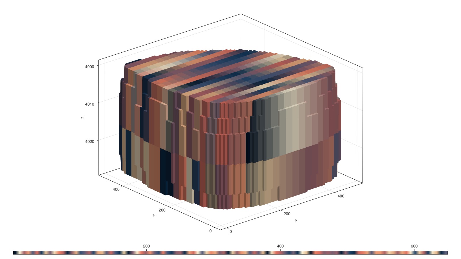
Compare fine-scale and coarse-scale permeability
The fine-scale and coarse-scale permeability fields are compared visually. The coarsening uses a static upscaling, where the permeability is harmonically averaged per direction when coarsening. This is a simple method that can be effective enough for many cases.
The fine-scale permeability is shown on the left, and the coarse-scale is shown on the right, with the same color axis.
K_f = fine_reservoir[:permeability][1, :]
K_c = coarse_reservoir[:permeability][1, :]

kcaxis = extrema(K_f)

fig = Figure(size = (1200, 500))
axf = Axis3(fig[1, 1], title = "Fine scale permeability", zreversed = true)
plot_cell_data!(axf, fine_mesh, K_f, colorrange = kcaxis, colormap = :turbo)

axc = Axis3(fig[1, 2], title = "Coarse scale permeability", zreversed = true)
plt = plot_cell_data!(axc, coarse_mesh, K_c, colorrange = kcaxis, colormap = :turbo)
Colorbar(fig[1, 3], plt)
fig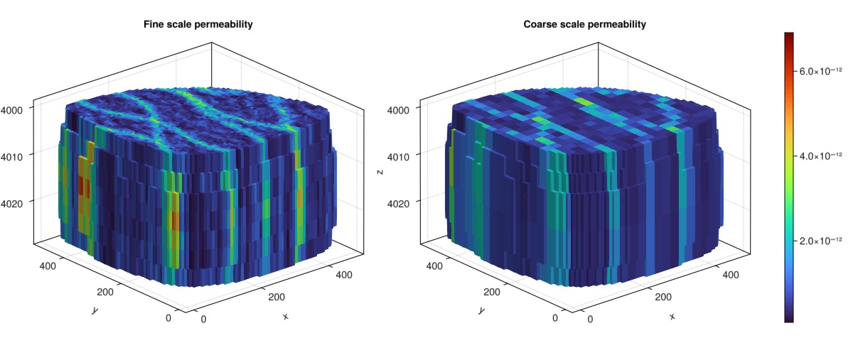
Simulate the coarse-scale model
The coarse scale model can be simulated just as the fine-scale model was, but the runtime should be significantly reduced down to around a second.
@time ws_c, states_c = simulate_reservoir(coarse_case, info_level = -1); 1.191235 seconds (4.02 M allocations: 318.147 MiB, 6.96% gc time)Plot and compare the coarse-scale and fine-scale solutions
We plot the pressure field for the fine-scale and coarse-scale models. The model has little pressure variation, but we see that there are substantial differences between our very coarse model and the original fine-scale.
using Statistics
wells = JutulDarcy.get_model_wells(fine_model)

p_c = states_c[end][:Pressure]
p_f = states[end][:Pressure]

caxis = extrema([extrema(p_c)..., extrema(p_f)...])

fig = Figure(size = (1200, 500))
axf = Axis3(fig[1, 1], title = "Fine scale", zreversed = true)
plot_cell_data!(axf, fine_mesh, p_f, colorrange = caxis, colormap = :turbo)

for (k, w) in wells
    plot_well!(axf, fine_mesh, w, fontsize = 0)
end

axc = Axis3(fig[1, 2], title = "Coarse scale", zreversed = true)
plt = plot_cell_data!(axc, coarse_mesh, p_c, colorrange = caxis, colormap = :turbo)

for (k, w) in wells
    plot_well!(axc, fine_mesh, w, fontsize = 0)
end
Colorbar(fig[1, 3], plt)
fig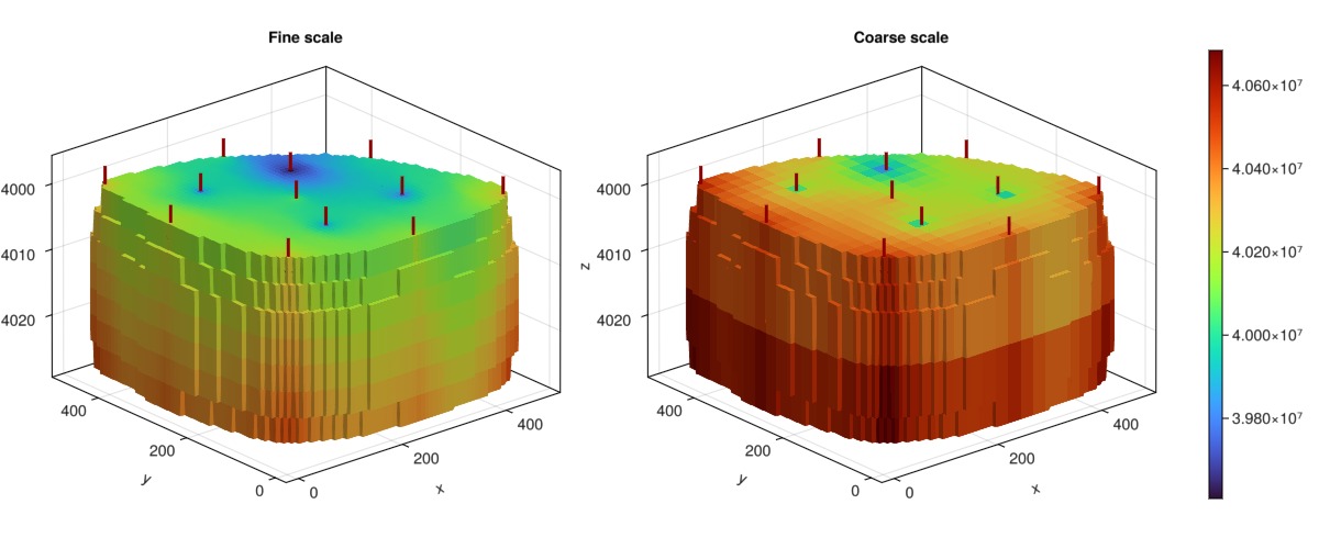
Plot and compare the saturation fields
We observe that the saturation fields are quite different between the coarse-scale and fine scale, with the coarse-scale model showing a more uniform saturation field as the leading shock is smeared away.
s_c = states_c[end][:Saturations][1, :]
s_f = states[end][:Saturations][1, :]

scaxis = extrema([extrema(s_c)..., extrema(s_f)...])

fig = Figure(size = (1200, 500))
axf = Axis3(fig[1, 1], title = "Fine scale", zreversed = true)
plot_cell_data!(axf, fine_mesh, s_f, colorrange = scaxis, colormap = :turbo)

for (k, w) in wells
    plot_well!(axf, fine_mesh, w, fontsize = 0)
end

axc = Axis3(fig[1, 2], title = "Coarse scale", zreversed = true)
plt = plot_cell_data!(axc, coarse_mesh, s_c, colorrange = scaxis, colormap = :turbo)

for (k, w) in wells
    plot_well!(axc, fine_mesh, w, fontsize = 0)
end
Colorbar(fig[1, 3], plt)
fig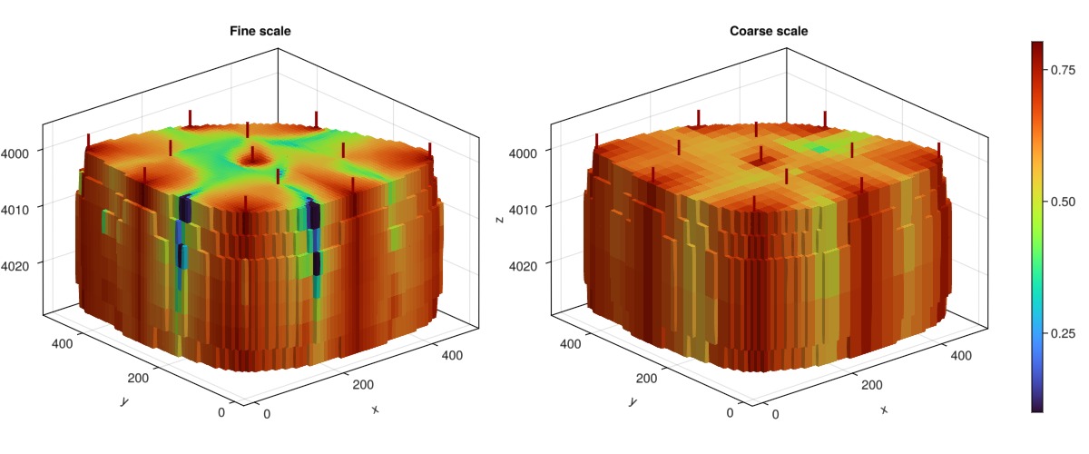
Plot the average field scale pressure evolution
fig = Figure()
axf_p = Axis(fig[1, 1], ylabel = "Avg. pressure / bar")
lines!(axf_p, map(x -> mean(x[:Pressure])/1e5, states), label = "Fine")
lines!(axf_p, map(x -> mean(x[:Pressure])/1e5, states_c), label = "Coarse")
axislegend()
fig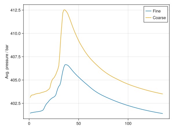
Plot the wells interactively
We can plot the well results in the interactive viewer using the comparison feature that allows multiple results to be superimposed in the same figure.
plot_well_results([ws, ws_c], names = ["Fine", "Coarse"], field = :orat, accumulated = true)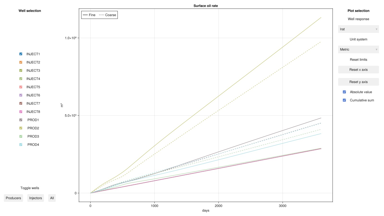
Plot field scale measurables over time interactively
The field-scale quantities match fairly well between the coarse-scale and fine-scale models. There is always a trade-off between accuracy and quality in numerical simulations, where the goal is to find the right balance between accuracy in quantities of interest and computational cost.
fine_m = reservoir_measurables(fine_case, ws, states)
coarse_m = reservoir_measurables(coarse_case, ws_c, states_c)
m = copy(fine_m)
for (k, v) in pairs(coarse_m)
    if k != :time
        m[Symbol("coarse_$k")] = v
    end
end

plot_reservoir_measurables(m, left = :fopr, right = :coarse_fopr, accumulated = true)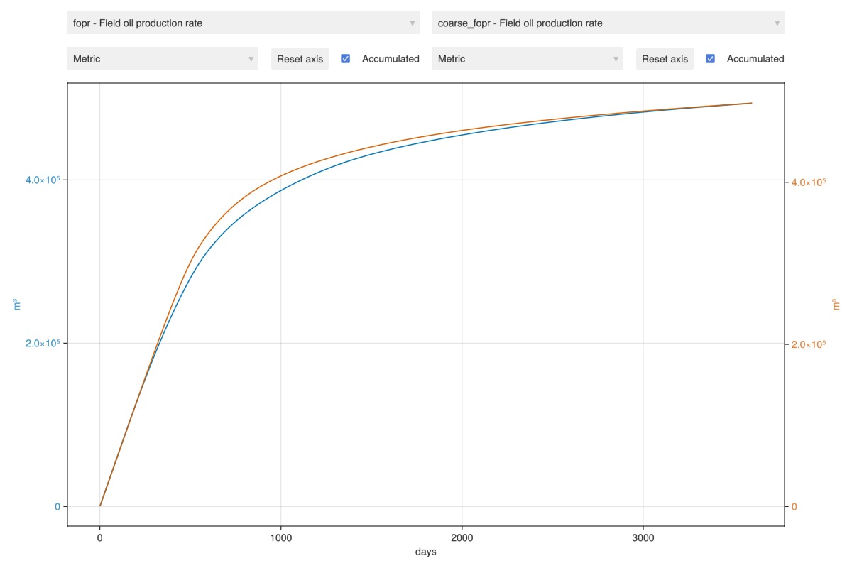
Compare different partitioning methods
We have only so far tested a single partitioning method. We can quickly generate a few other coarse models using different partitioning methods and coarsening values. We highlight that we can also use the centroids instead of the IJK indices to partition, for when the mesh may not have a structured background mesh. In addition, we can call different graph partitioners by passing the desired number of blocks. Here, we call a simple METIS-based transmissibility coarsening, but the code contains options to use other weights and partitioners.
partition_variants = [
    (:centroids, (3, 3, 2)),
    (:ijk, (5, 5, 1)),
    (:metis, 10),
    (:metis, 50)
]

fig = Figure(size = (1200, 600))
layout = GridLayout()
fig[1, 1] = layout
rowwidth = Int(floor(length(partition_variants)/2))
for (no, variant) in enumerate(partition_variants)
    if no > rowwidth
        row = 2
        pix = no - rowwidth
    else
        row = 1
        pix = no
    end
    cmethod, cdim = variant
    variant_case = coarsen_reservoir_case(fine_case, cdim, method = cmethod)
    r = reservoir_domain(variant_case)
    m = physical_representation(r)
    p = m.partition

    ax = Axis3(fig, title = "$cmethod - $cdim", azimuth = 0.3, elevation = 1.0, zreversed = true)
    plot_cell_data!(ax, fine_mesh, p, colormap = :lipariS)
    layout[row, 2*(pix-1) + 1] = ax

    _, variant_states = simulate_reservoir(variant_case, info_level = -1)
    pres = variant_states[end][:Pressure]
    axp = Axis3(fig, title = "Pressure", azimuth = 0.3, elevation = 1.0, zreversed = true)
    for (k, w) in wells
        plot_well!(axp, fine_mesh, w, fontsize = 0)
    end
    plot_cell_data!(axp, m, pres, colorrange = caxis, colormap = :turbo)

    layout[row, 2*(pix-1) + 2] = axp
end
fig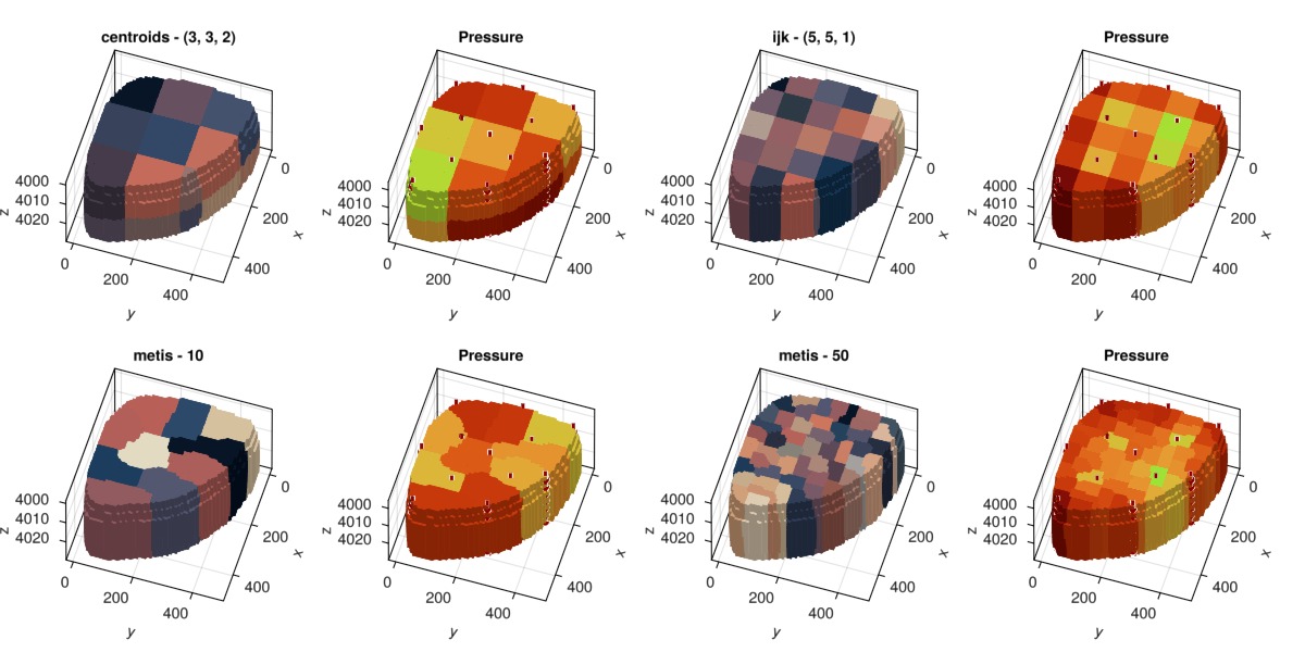
Example on GitHub
If you would like to run this example yourself, it can be downloaded from the JutulDarcy.jl GitHub repository as a script, or as a Jupyter Notebook
This page was generated using Literate.jl.