Example demonstrating compositional flow

This is a simple conceptual example demonstrating how to solve compositional flow. This example uses a two-component water-CO2 system. Note that the default Peng-Robinson is not accurate for this system without adjustments to the parameters. However, the example demonstrates the conceptual workflow for getting started with compositional simulation.

Set up mixture

We load the external flash package and define a two-component H2O-CO2 system. The constructor for each species takes in molecular weight, critical pressure, critical temperature, critical volume, acentric factor given as strict SI. This means, for instance, that molar masses are given in kg/mole and not g/mole or kg/kmol.

using MultiComponentFlash
h2o = MolecularProperty(0.018015268, 22.064e6, 647.096, 5.595e-05, 0.3442920843)
co2 = MolecularProperty(0.0440098, 7.3773e6, 304.1282, 9.412e-05, 0.22394)

bic = zeros(2, 2)

mixture = MultiComponentMixture([h2o, co2], A_ij = bic, names = ["H2O", "CO2"])
eos = GenericCubicEOS(mixture, PengRobinson())

MultiComponentFlash.GenericCubicEOS{MultiComponentFlash.PengRobinson, Float64, 2, Nothing}(MultiComponentFlash.PengRobinson(), MultiComponentFlash.MultiComponentMixture{Float64, 2}("UnnamedMixture", ["H2O", "CO2"], (MultiComponentFlash.MolecularProperty{Float64}(0.018015268, 2.2064e7, 647.096, 5.595e-5, 0.3442920843), MultiComponentFlash.MolecularProperty{Float64}(0.0440098, 7.3773e6, 304.1282, 9.412e-5, 0.22394)), [0.0 0.0; 0.0 0.0]), 2.414213562373095, -0.41421356237309515, 0.457235529, 0.077796074, nothing)

Set up domain and wells

using Jutul, JutulDarcy, GLMakie
nx = 50
ny = 1
nz = 20
dims = (nx, ny, nz)
g = CartesianMesh(dims, (100.0, 10.0, 10.0))
nc = number_of_cells(g)
Darcy, bar, kg, meter, Kelvin, day, sec = si_units(:darcy, :bar, :kilogram, :meter, :Kelvin, :day, :second)
K = repeat([0.1, 0.1, 0.001]*Darcy, 1, nc)
res = reservoir_domain(g, porosity = 0.3, permeability = K)

DataDomain wrapping CartesianMesh (3D) with 50x1x20=1000 cells with 17 data fields added:
  1000 Cells
    :permeability => 3×1000 Matrix{Float64}
    :porosity => 1000 Vector{Float64}
    :rock_thermal_conductivity => 1000 Vector{Float64}
    :fluid_thermal_conductivity => 1000 Vector{Float64}
    :rock_density => 1000 Vector{Float64}
    :cell_centroids => 3×1000 Matrix{Float64}
    :volumes => 1000 Vector{Float64}
  1930 Faces
    :neighbors => 2×1930 Matrix{Int64}
    :areas => 1930 Vector{Float64}
    :normals => 3×1930 Matrix{Float64}
    :face_centroids => 3×1930 Matrix{Float64}
  3860 HalfFaces
    :half_face_cells => 3860 Vector{Int64}
    :half_face_faces => 3860 Vector{Int64}
  2140 BoundaryFaces
    :boundary_areas => 2140 Vector{Float64}
    :boundary_centroids => 3×2140 Matrix{Float64}
    :boundary_normals => 3×2140 Matrix{Float64}
    :boundary_neighbors => 2140 Vector{Int64}

Set up a vertical well in the first corner, perforated in top layer

prod = setup_well(g, K, [(nx, ny, 1)], name = :Producer)

MultiSegmentWell [Producer] (2 nodes, 1 segments, 1 perforations)

Set up an injector in the opposite corner, perforated in bottom layer

inj = setup_well(g, K, [(1, 1, nz)], name = :Injector)

MultiSegmentWell [Injector] (2 nodes, 1 segments, 1 perforations)

Define system and realize on grid

rhoLS = 844.23*kg/meter^3
rhoVS = 126.97*kg/meter^3
rhoS = [rhoLS, rhoVS]
L, V = LiquidPhase(), VaporPhase()
sys = MultiPhaseCompositionalSystemLV(eos, (L, V))
model, parameters = setup_reservoir_model(res, sys, wells = [inj, prod]);
push!(model[:Reservoir].output_variables, :Saturations)
kr = BrooksCoreyRelativePermeabilities(sys, 2.0, 0.0, 1.0)
model = replace_variables!(model, RelativePermeabilities = kr)
T0 = fill(303.15*Kelvin, nc)
parameters[:Reservoir][:Temperature] = T0
state0 = setup_reservoir_state(model, Pressure = 50*bar, OverallMoleFractions = [1.0, 0.0]);

Define schedule

5 year (5*365.24 days) simulation period

dt0 = fill(1*day, 26)
dt1 = fill(10.0*day, 180)
dt = cat(dt0, dt1, dims = 1)
rate_target = TotalRateTarget(9.5066e-06*meter^3/sec)
I_ctrl = InjectorControl(rate_target, [0, 1], density = rhoVS)
bhp_target = BottomHolePressureTarget(50*bar)
P_ctrl = ProducerControl(bhp_target)

controls = Dict()
controls[:Injector] = I_ctrl
controls[:Producer] = P_ctrl
forces = setup_reservoir_forces(model, control = controls)
ws, states = simulate_reservoir(state0, model, dt, parameters = parameters, forces = forces)

ReservoirSimResult with 206 entries:

  wells (2 present):
    :Producer
    :Injector
    Results per well:
       :H2O_mass_rate => Vector{Float64} of size (206,)
       :lrat => Vector{Float64} of size (206,)
       :orat => Vector{Float64} of size (206,)
       :control => Vector{Symbol} of size (206,)
       :bhp => Vector{Float64} of size (206,)
       :CO2_mass_rate => Vector{Float64} of size (206,)
       :mass_rate => Vector{Float64} of size (206,)
       :rate => Vector{Float64} of size (206,)
       :grat => Vector{Float64} of size (206,)
       :gor => Vector{Float64} of size (206,)

  states (Vector with 206 entries, reservoir variables for each state)
    :LiquidMassFractions => Matrix{Float64} of size (2, 1000)
    :OverallMoleFractions => Matrix{Float64} of size (2, 1000)
    :Saturations => Matrix{Float64} of size (2, 1000)
    :Pressure => Vector{Float64} of size (1000,)
    :VaporMassFractions => Matrix{Float64} of size (2, 1000)
    :TotalMasses => Matrix{Float64} of size (2, 1000)

  time (report time for each state)
     Vector{Float64} of length 206

  result (extended states, reports)
     SimResult with 206 entries

  extra
     Dict{Any, Any} with keys :simulator, :config

  Completed at Oct. 15 2024 11:10 after 13 seconds, 552 milliseconds, 442.8 microseconds.

Once the simulation is done, we can plot the states

Note that this example is intended for static publication in the documentation. For interactive visualization you can use functions like plot_interactive to interactively visualize the states.

z = states[end][:OverallMoleFractions][2, :]
function plot_vertical(x, t)
    data = reshape(x, (nx, nz))
    data = data[:, end:-1:1]
    fig, ax, plot = heatmap(data)
    ax.title = t
    Colorbar(fig[1, 2], plot)
    fig
end

plot_vertical (generic function with 1 method)

Plot final CO2 mole fraction

plot_vertical(z, "CO2")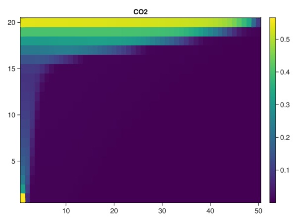

Plot final vapor saturation

sg = states[end][:Saturations][2, :]
plot_vertical(sg, "Vapor saturation")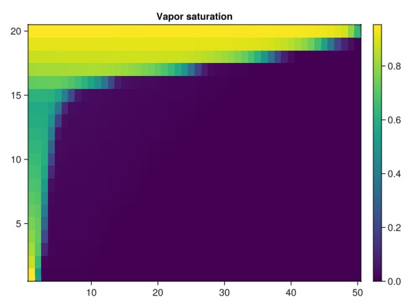

Plot final pressure

p = states[end][:Pressure]
plot_vertical(p./bar, "Pressure [bar]")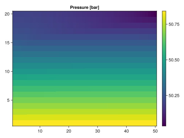

Plot in interactive viewer

plot_reservoir(model, states, step = length(dt), key = :Saturations)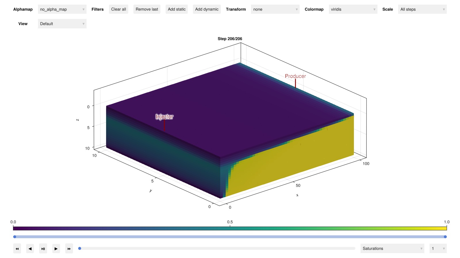

Example on GitHub

If you would like to run this example yourself, it can be downloaded from the JutulDarcy.jl GitHub repository as a script, or as a Jupyter Notebook

---

This page was generated using Literate.jl.