History matching a coarse model - CGNet

This example demonstrates how to calibrate a coarse model against results from a fine model. We do this by optimizing the parameters of the coarse model to match the well curves. This is a implementation of the method described in [7]. This also serves as a demonstration of how to use the simulator for history matching, as the fine model results can stand in for real field observations.

Load and simulate Egg base case

julia

using Jutul, JutulDarcy, HYPRE, GeoEnergyIO, GLMakie
import LBFGSB as lb

egg_dir = JutulDarcy.GeoEnergyIO.test_input_file_path("EGG")
data_pth = joinpath(egg_dir, "EGG.DATA")

fine_case = setup_case_from_data_file(data_pth)
simulated_fine = simulate_reservoir(fine_case)
plot_reservoir(fine_case, simulated_fine.states, key = :Saturations, step = 100)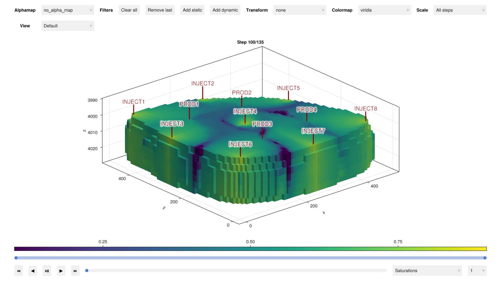

Create initial coarse model and simulate

julia

coarse_case = JutulDarcy.coarsen_reservoir_case(fine_case, (25, 25, 5), method = :ijk)
simulated_coarse = simulate_reservoir(coarse_case, info_level = -1)
plot_reservoir(coarse_case, simulated_coarse.states, key = :Saturations, step = 100)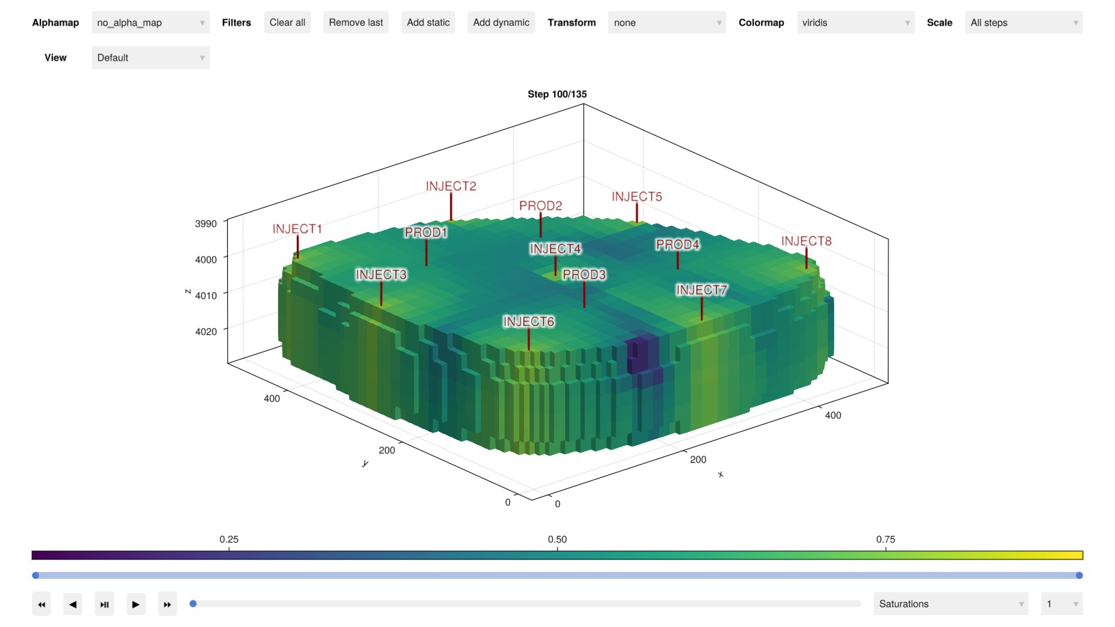

Setup optimization

We set up the optimization problem by defining the objective function as a sum of squared mismatches for all well observations, for all time-steps. We also define limits for the parameters, and set up the optimization problem.

julia

function setup_optimization_cgnet(case_c, case_f, result_f)
    states_f = result_f.result.states
    wells_results, = result_f
    model_c = case_c.model
    state0_c = setup_state(model_c, case_c.state0);
    param_c = setup_parameters(model_c)
    forces_c = case_c.forces
    dt = case_c.dt
    model_f = case_f.model

    bhp = JutulDarcy.BottomHolePressureTarget(1.0)
    wells = collect(keys(JutulDarcy.get_model_wells(case_f)))

    day = si_unit(:day)
    wrat_scale = (1/150)*day
    orat_scale = (1/80)*day
    grat_scale = (1/1000)*day

    w = []
    matches = []
    signs = []
    sys = reservoir_model(model_f).system
    wrat = SurfaceWaterRateTarget(-1.0)
    orat = SurfaceOilRateTarget(-1.0)
    grat = SurfaceGasRateTarget(-1.0)

    push!(matches, bhp)
    push!(w, 1.0/si_unit(:bar))
    push!(signs, 1)

    for phase in JutulDarcy.get_phases(sys)
        if phase == LiquidPhase()
            push!(matches, orat)
            push!(w, orat_scale)
            push!(signs, -1)

        elseif phase == VaporPhase()
            push!(matches, grat)
            push!(w, grat_scale)
            push!(signs, -1)
        else
            @assert phase == AqueousPhase()
            push!(matches, wrat)
            push!(w, wrat_scale)
            push!(signs, -1)
        end
    end
    signs = zeros(Int, length(signs))
    o_scale = 1.0/(sum(dt)*length(wells))
    G = (model_c, state_c, dt, step_no, forces) -> well_mismatch(
        matches,
        wells,
        model_f,
        states_f,
        model_c,
        state_c,
        dt,
        step_no,
        forces,
        weights = w,
        scale = o_scale,
        signs = signs
    )

    @assert Jutul.evaluate_objective(G, model_f, states_f, dt, case_f.forces) == 0.0
    #
    cfg = optimization_config(model_c, param_c,
        use_scaling = true,
        rel_min = 0.001,
        rel_max = 1000
    )
    for (k, v) in cfg
        for (ki, vi) in v
            if ki == :FluidVolume
                vi[:active] = k == :Reservoir
            end
            if ki == :ConnateWater
                vi[:active] = false
            end
            if ki in [:TwoPointGravityDifference, :PhaseViscosities, :PerforationGravityDifference]
                vi[:active] = false
            end
            if ki in [:WellIndices, :Transmissibilities]
                vi[:active] = true
                vi[:abs_min] = 0.0
                vi[:abs_max] = 1e-6
            end

        end
    end
    opt_setup = setup_parameter_optimization(model_c, state0_c, param_c, dt, forces_c, G, cfg);
    x0 = opt_setup.x0
    F0 = opt_setup.F!(x0)
    dF0 = opt_setup.dF!(similar(x0), x0)
    println("Initial objective: $F0, gradient norm $(sum(abs, dF0))")
    return opt_setup
end

setup_optimization_cgnet (generic function with 1 method)

Define the optimization loop

JutulDarcy can use any optimization package that can work with gradients and limits, here we use the LBFGSB package.

julia

function optimize_cgnet(opt_setup)
    lower = opt_setup.limits.min
    upper = opt_setup.limits.max
    x0 = opt_setup.x0
    n = length(x0)
    setup = Dict(:lower => lower, :upper => upper, :x0 => copy(x0))

    prt = 1
    f! = (x) -> opt_setup.F_and_dF!(NaN, nothing, x)
    g! = (dFdx, x) -> opt_setup.F_and_dF!(NaN, dFdx, x)
    results, final_x = lb.lbfgsb(f!, g!, x0, lb=lower, ub=upper,
        iprint = prt,
        factr = 1e12,
        maxfun = 50,
        maxiter = 50,
        m = 20
    )
    return (final_x, results, setup)
end

optimize_cgnet (generic function with 1 method)

Run the optimization

julia

opt_setup = setup_optimization_cgnet(coarse_case, fine_case, simulated_fine);
final_x, results, setup = optimize_cgnet(opt_setup);

Parameters for PROD4
┌─────────────┬──────────────┬───┬─────────┬─────────────┬────────────────┬──────────────────────┬─────────┐
│        Name │       Entity │ N │   Scale │ Abs. limits │    Rel. limits │               Limits │ Lumping │
├─────────────┼──────────────┼───┼─────────┼─────────────┼────────────────┼──────────────────────┼─────────┤
│ WellIndices │ Perforations │ 5 │ default │  [0, 1e-06] │ [0.001, 1e+03] │ [4.22e-15, 7.95e-09] │       - │
└─────────────┴──────────────┴───┴─────────┴─────────────┴────────────────┴──────────────────────┴─────────┘
Parameters for Reservoir
┌────────────────────┬────────┬──────┬─────────┬─────────────────┬────────────────┬──────────────────────┬─────────┐
│               Name │ Entity │    N │   Scale │     Abs. limits │    Rel. limits │               Limits │ Lumping │
├────────────────────┼────────┼──────┼─────────┼─────────────────┼────────────────┼──────────────────────┼─────────┤
│ Transmissibilities │  Faces │ 6792 │ default │      [0, 1e-06] │ [0.001, 1e+03] │ [1.71e-16, 4.75e-08] │       - │
│        FluidVolume │  Cells │ 2516 │ default │ [2.22e-16, Inf] │ [0.001, 1e+03] │   [0.0512, 9.22e+05] │       - │
└────────────────────┴────────┴──────┴─────────┴─────────────────┴────────────────┴──────────────────────┴─────────┘
Parameters for INJECT5
┌─────────────┬──────────────┬───┬─────────┬─────────────┬────────────────┬──────────────────────┬─────────┐
│        Name │       Entity │ N │   Scale │ Abs. limits │    Rel. limits │               Limits │ Lumping │
├─────────────┼──────────────┼───┼─────────┼─────────────┼────────────────┼──────────────────────┼─────────┤
│ WellIndices │ Perforations │ 5 │ default │  [0, 1e-06] │ [0.001, 1e+03] │ [9.46e-15, 1.96e-08] │       - │
└─────────────┴──────────────┴───┴─────────┴─────────────┴────────────────┴──────────────────────┴─────────┘
Parameters for INJECT4
┌─────────────┬──────────────┬───┬─────────┬─────────────┬────────────────┬──────────────────────┬─────────┐
│        Name │       Entity │ N │   Scale │ Abs. limits │    Rel. limits │               Limits │ Lumping │
├─────────────┼──────────────┼───┼─────────┼─────────────┼────────────────┼──────────────────────┼─────────┤
│ WellIndices │ Perforations │ 5 │ default │  [0, 1e-06] │ [0.001, 1e+03] │ [2.33e-15, 5.35e-09] │       - │
└─────────────┴──────────────┴───┴─────────┴─────────────┴────────────────┴──────────────────────┴─────────┘
Parameters for INJECT8
┌─────────────┬──────────────┬───┬─────────┬─────────────┬────────────────┬─────────────────────┬─────────┐
│        Name │       Entity │ N │   Scale │ Abs. limits │    Rel. limits │              Limits │ Lumping │
├─────────────┼──────────────┼───┼─────────┼─────────────┼────────────────┼─────────────────────┼─────────┤
│ WellIndices │ Perforations │ 5 │ default │  [0, 1e-06] │ [0.001, 1e+03] │ [2.9e-15, 7.68e-09] │       - │
└─────────────┴──────────────┴───┴─────────┴─────────────┴────────────────┴─────────────────────┴─────────┘
Parameters for INJECT6
┌─────────────┬──────────────┬───┬─────────┬─────────────┬────────────────┬──────────────────────┬─────────┐
│        Name │       Entity │ N │   Scale │ Abs. limits │    Rel. limits │               Limits │ Lumping │
├─────────────┼──────────────┼───┼─────────┼─────────────┼────────────────┼──────────────────────┼─────────┤
│ WellIndices │ Perforations │ 5 │ default │  [0, 1e-06] │ [0.001, 1e+03] │ [5.94e-15, 1.29e-08] │       - │
└─────────────┴──────────────┴───┴─────────┴─────────────┴────────────────┴──────────────────────┴─────────┘
Parameters for INJECT1
┌─────────────┬──────────────┬───┬─────────┬─────────────┬────────────────┬──────────────────────┬─────────┐
│        Name │       Entity │ N │   Scale │ Abs. limits │    Rel. limits │               Limits │ Lumping │
├─────────────┼──────────────┼───┼─────────┼─────────────┼────────────────┼──────────────────────┼─────────┤
│ WellIndices │ Perforations │ 5 │ default │  [0, 1e-06] │ [0.001, 1e+03] │ [4.45e-15, 1.02e-08] │       - │
└─────────────┴──────────────┴───┴─────────┴─────────────┴────────────────┴──────────────────────┴─────────┘
Parameters for INJECT7
┌─────────────┬──────────────┬───┬─────────┬─────────────┬────────────────┬──────────────────────┬─────────┐
│        Name │       Entity │ N │   Scale │ Abs. limits │    Rel. limits │               Limits │ Lumping │
├─────────────┼──────────────┼───┼─────────┼─────────────┼────────────────┼──────────────────────┼─────────┤
│ WellIndices │ Perforations │ 5 │ default │  [0, 1e-06] │ [0.001, 1e+03] │ [2.23e-15, 4.66e-09] │       - │
└─────────────┴──────────────┴───┴─────────┴─────────────┴────────────────┴──────────────────────┴─────────┘
Parameters for INJECT3
┌─────────────┬──────────────┬───┬─────────┬─────────────┬────────────────┬─────────────────────┬─────────┐
│        Name │       Entity │ N │   Scale │ Abs. limits │    Rel. limits │              Limits │ Lumping │
├─────────────┼──────────────┼───┼─────────┼─────────────┼────────────────┼─────────────────────┼─────────┤
│ WellIndices │ Perforations │ 5 │ default │  [0, 1e-06] │ [0.001, 1e+03] │ [4.87e-15, 1.3e-08] │       - │
└─────────────┴──────────────┴───┴─────────┴─────────────┴────────────────┴─────────────────────┴─────────┘
Parameters for PROD2
┌─────────────┬──────────────┬───┬─────────┬─────────────┬────────────────┬──────────────────────┬─────────┐
│        Name │       Entity │ N │   Scale │ Abs. limits │    Rel. limits │               Limits │ Lumping │
├─────────────┼──────────────┼───┼─────────┼─────────────┼────────────────┼──────────────────────┼─────────┤
│ WellIndices │ Perforations │ 5 │ default │  [0, 1e-06] │ [0.001, 1e+03] │ [2.96e-14, 4.31e-08] │       - │
└─────────────┴──────────────┴───┴─────────┴─────────────┴────────────────┴──────────────────────┴─────────┘
Parameters for PROD3
┌─────────────┬──────────────┬───┬─────────┬─────────────┬────────────────┬─────────────────────┬─────────┐
│        Name │       Entity │ N │   Scale │ Abs. limits │    Rel. limits │              Limits │ Lumping │
├─────────────┼──────────────┼───┼─────────┼─────────────┼────────────────┼─────────────────────┼─────────┤
│ WellIndices │ Perforations │ 5 │ default │  [0, 1e-06] │ [0.001, 1e+03] │ [2.34e-15, 5.7e-09] │       - │
└─────────────┴──────────────┴───┴─────────┴─────────────┴────────────────┴─────────────────────┴─────────┘
Parameters for PROD1
┌─────────────┬──────────────┬───┬─────────┬─────────────┬────────────────┬──────────────────────┬─────────┐
│        Name │       Entity │ N │   Scale │ Abs. limits │    Rel. limits │               Limits │ Lumping │
├─────────────┼──────────────┼───┼─────────┼─────────────┼────────────────┼──────────────────────┼─────────┤
│ WellIndices │ Perforations │ 5 │ default │  [0, 1e-06] │ [0.001, 1e+03] │ [2.04e-15, 4.29e-09] │       - │
└─────────────┴──────────────┴───┴─────────┴─────────────┴────────────────┴──────────────────────┴─────────┘
Parameters for INJECT2
┌─────────────┬──────────────┬───┬─────────┬─────────────┬────────────────┬──────────────────────┬─────────┐
│        Name │       Entity │ N │   Scale │ Abs. limits │    Rel. limits │               Limits │ Lumping │
├─────────────┼──────────────┼───┼─────────┼─────────────┼────────────────┼──────────────────────┼─────────┤
│ WellIndices │ Perforations │ 5 │ default │  [0, 1e-06] │ [0.001, 1e+03] │ [1.08e-14, 2.15e-08] │       - │
└─────────────┴──────────────┴───┴─────────┴─────────────┴────────────────┴──────────────────────┴─────────┘
#1: 3.7373302810581173
Initial objective: 3.7373302810581173, gradient norm 2.983773972465357e6
RUNNING THE L-BFGS-B CODE

           * * *

Machine precision = 2.220D-16
 N =         9368     M =           20

At X0         0 variables are exactly at the bounds

At iterate    0    f=  3.73733D+00    |proj g|=  9.99001D-01
┌ Warning: Partial data passed, objective set to large value 37.37330281058117.
└ @ Jutul ~/.julia/packages/Jutul/VbNFh/src/ad/gradients.jl:682
#2: 37.37330281058117
[31;1mPROD1:[0m Approaching zero rate, disabling producer for current step
[31;1mPROD1:[0m Approaching zero rate, disabling producer for current step
[31;1mPROD1:[0m Approaching zero rate, disabling producer for current step
[31;1mPROD1:[0m Approaching zero rate, disabling producer for current step
[31;1mPROD1:[0m Approaching zero rate, disabling producer for current step
[31;1mPROD1:[0m Approaching zero rate, disabling producer for current step
[31;1mPROD1:[0m Approaching zero rate, disabling producer for current step
[31;1mPROD1:[0m Approaching zero rate, disabling producer for current step
[31;1mPROD1:[0m Approaching zero rate, disabling producer for current step
[31;1mPROD1:[0m Approaching zero rate, disabling producer for current step
[31;1mPROD1:[0m Approaching zero rate, disabling producer for current step
[31;1mPROD1:[0m Approaching zero rate, disabling producer for current step
[31;1mPROD1:[0m Approaching zero rate, disabling producer for current step
[31;1mPROD1:[0m Approaching zero rate, disabling producer for current step
[31;1mPROD1:[0m Approaching zero rate, disabling producer for current step
[31;1mPROD1:[0m Approaching zero rate, disabling producer for current step
[31;1mPROD1:[0m Approaching zero rate, disabling producer for current step
[31;1mPROD1:[0m Approaching zero rate, disabling producer for current step
[31;1mPROD1:[0m Approaching zero rate, disabling producer for current step
[31;1mPROD1:[0m Approaching zero rate, disabling producer for current step
[31;1mPROD1:[0m Approaching zero rate, disabling producer for current step
[31;1mPROD1:[0m Approaching zero rate, disabling producer for current step
[31;1mPROD1:[0m Approaching zero rate, disabling producer for current step
[31;1mPROD1:[0m Approaching zero rate, disabling producer for current step
[31;1mPROD1:[0m Approaching zero rate, disabling producer for current step
[31;1mPROD1:[0m Approaching zero rate, disabling producer for current step
[31;1mPROD1:[0m Approaching zero rate, disabling producer for current step
[31;1mPROD1:[0m Approaching zero rate, disabling producer for current step
[31;1mPROD1:[0m Approaching zero rate, disabling producer for current step
[31;1mPROD1:[0m Approaching zero rate, disabling producer for current step
[31;1mPROD1:[0m Approaching zero rate, disabling producer for current step
[31;1mPROD1:[0m Approaching zero rate, disabling producer for current step
[31;1mPROD1:[0m Approaching zero rate, disabling producer for current step
[31;1mPROD1:[0m Approaching zero rate, disabling producer for current step
[31;1mPROD1:[0m Approaching zero rate, disabling producer for current step
[31;1mPROD1:[0m Approaching zero rate, disabling producer for current step
[31;1mPROD1:[0m Approaching zero rate, disabling producer for current step
[31;1mPROD1:[0m Approaching zero rate, disabling producer for current step
[31;1mPROD1:[0m Approaching zero rate, disabling producer for current step
[31;1mPROD1:[0m Approaching zero rate, disabling producer for current step
[31;1mPROD1:[0m Approaching zero rate, disabling producer for current step
[31;1mPROD1:[0m Approaching zero rate, disabling producer for current step
[31;1mPROD1:[0m Approaching zero rate, disabling producer for current step
[31;1mPROD1:[0m Approaching zero rate, disabling producer for current step
[31;1mPROD1:[0m Approaching zero rate, disabling producer for current step
[31;1mPROD1:[0m Approaching zero rate, disabling producer for current step
[31;1mPROD1:[0m Approaching zero rate, disabling producer for current step
[31;1mPROD1:[0m Approaching zero rate, disabling producer for current step
[31;1mPROD1:[0m Approaching zero rate, disabling producer for current step
[31;1mPROD1:[0m Approaching zero rate, disabling producer for current step
[31;1mPROD1:[0m Approaching zero rate, disabling producer for current step
[31;1mPROD1:[0m Approaching zero rate, disabling producer for current step
[31;1mPROD1:[0m Approaching zero rate, disabling producer for current step
[31;1mPROD1:[0m Approaching zero rate, disabling producer for current step
[31;1mPROD1:[0m Approaching zero rate, disabling producer for current step
[31;1mPROD1:[0m Approaching zero rate, disabling producer for current step
[31;1mPROD1:[0m Approaching zero rate, disabling producer for current step
[31;1mPROD1:[0m Approaching zero rate, disabling producer for current step
[31;1mPROD1:[0m Approaching zero rate, disabling producer for current step
[31;1mPROD1:[0m Approaching zero rate, disabling producer for current step
[31;1mPROD1:[0m Approaching zero rate, disabling producer for current step
[31;1mPROD1:[0m Approaching zero rate, disabling producer for current step
[31;1mPROD1:[0m Approaching zero rate, disabling producer for current step
[31;1mPROD1:[0m Approaching zero rate, disabling producer for current step
[31;1mPROD1:[0m Approaching zero rate, disabling producer for current step
[31;1mPROD1:[0m Approaching zero rate, disabling producer for current step
[31;1mPROD1:[0m Approaching zero rate, disabling producer for current step
[31;1mPROD1:[0m Approaching zero rate, disabling producer for current step
[31;1mPROD1:[0m Approaching zero rate, disabling producer for current step
[31;1mPROD1:[0m Approaching zero rate, disabling producer for current step
[31;1mPROD1:[0m Approaching zero rate, disabling producer for current step
[31;1mPROD1:[0m Approaching zero rate, disabling producer for current step
[31;1mPROD1:[0m Approaching zero rate, disabling producer for current step
[31;1mPROD1:[0m Approaching zero rate, disabling producer for current step
#3: 65.01329948286727
[31;1mPROD1:[0m Approaching zero rate, disabling producer for current step
[31;1mPROD1:[0m Approaching zero rate, disabling producer for current step
[31;1mPROD1:[0m Approaching zero rate, disabling producer for current step
[31;1mPROD1:[0m Approaching zero rate, disabling producer for current step
[31;1mPROD1:[0m Approaching zero rate, disabling producer for current step
[31;1mPROD1:[0m Approaching zero rate, disabling producer for current step
[31;1mPROD1:[0m Approaching zero rate, disabling producer for current step
[31;1mPROD1:[0m Approaching zero rate, disabling producer for current step
[31;1mPROD1:[0m Approaching zero rate, disabling producer for current step
[31;1mPROD1:[0m Approaching zero rate, disabling producer for current step
[31;1mPROD1:[0m Approaching zero rate, disabling producer for current step
[31;1mPROD1:[0m Approaching zero rate, disabling producer for current step
[31;1mPROD1:[0m Approaching zero rate, disabling producer for current step
[31;1mPROD1:[0m Approaching zero rate, disabling producer for current step
[31;1mPROD1:[0m Approaching zero rate, disabling producer for current step
[31;1mPROD1:[0m Approaching zero rate, disabling producer for current step
[31;1mPROD1:[0m Approaching zero rate, disabling producer for current step
[31;1mPROD1:[0m Approaching zero rate, disabling producer for current step
[31;1mPROD1:[0m Approaching zero rate, disabling producer for current step
[31;1mPROD1:[0m Approaching zero rate, disabling producer for current step
[31;1mPROD1:[0m Approaching zero rate, disabling producer for current step
[31;1mPROD1:[0m Approaching zero rate, disabling producer for current step
[31;1mPROD1:[0m Approaching zero rate, disabling producer for current step
[31;1mPROD1:[0m Approaching zero rate, disabling producer for current step
[31;1mPROD1:[0m Approaching zero rate, disabling producer for current step
[31;1mPROD1:[0m Approaching zero rate, disabling producer for current step
[31;1mPROD1:[0m Approaching zero rate, disabling producer for current step
[31;1mPROD1:[0m Approaching zero rate, disabling producer for current step
#4: 64.00312090479714
#5: 62.026116365306535
#6: 58.23201287244935
#7: 47.43573546600407
#8: 26.596516029209578
#9: 7.439002071214933
#10: 0.607355568500212

At iterate    1    f=  6.07356D-01    |proj g|=  9.99000D-01
#11: 0.2931232022816694

At iterate    2    f=  2.93123D-01    |proj g|=  9.99000D-01
#12: 0.19240938697830032

At iterate    3    f=  1.92409D-01    |proj g|=  9.99000D-01
#13: 0.17230182149941603

At iterate    4    f=  1.72302D-01    |proj g|=  9.99000D-01
#14: 0.16527387286412265
#15: 0.14215780529802266

At iterate    5    f=  1.42158D-01    |proj g|=  9.99000D-01
#16: 0.12780219191760642
#17: 0.12601119693104737

At iterate    6    f=  1.26011D-01    |proj g|=  9.99001D-01
#18: 0.11894041426445714

At iterate    7    f=  1.18940D-01    |proj g|=  9.99006D-01
#19: 0.1136723350787393

At iterate    8    f=  1.13672D-01    |proj g|=  9.99006D-01
#20: 0.10834286997692137

At iterate    9    f=  1.08343D-01    |proj g|=  9.99008D-01
#21: 0.10199837327697019
#22: 0.10355406443666638

At iterate   10    f=  1.03554D-01    |proj g|=  9.99009D-01
#23: 0.13838261788043027
#24: 0.09408207722006041

At iterate   11    f=  9.40821D-02    |proj g|=  9.99008D-01
#25: 0.09395968818850925

At iterate   12    f=  9.39597D-02    |proj g|=  9.99012D-01

           * * *

Tit   = total number of iterations
Tnf   = total number of function evaluations
Tnint = total number of segments explored during Cauchy searches
Skip  = number of BFGS updates skipped
Nact  = number of active bounds at final generalized Cauchy point
Projg = norm of the final projected gradient
F     = final function value

           * * *

   N    Tit     Tnf  Tnint  Skip  Nact     Projg        F
 9368     12     25   9379     0     0   9.990D-01   9.396D-02
  F =   9.3959688188509249E-002

CONVERGENCE: REL_REDUCTION_OF_F_<=_FACTR*EPSMCH

 Cauchy                time 3.998E-03 seconds.
 Subspace minimization time 3.845E-03 seconds.
 Line search           time 1.725E+02 seconds.

 Total User time 1.757E+02 seconds.

Transfer the results back

The optimization is generic and works on a single long vector that represents all our active parameters. We can devectorize this vector back into the nested representation used by the model itself and simulate.

julia

tuned_case = deepcopy(opt_setup.data[:case])
model_c = coarse_case.model
model_f = fine_case.model
param_c = tuned_case.parameters
data = opt_setup.data
devectorize_variables!(param_c, model_c, final_x, data[:mapper], config = data[:config])


simulated_tuned = simulate_reservoir(tuned_case, info_level = -1);

Plot the results interactively

julia

using GLMakie

wells_f, = simulated_fine
wells_c, = simulated_coarse
wells_t, states_t, time = simulated_tuned

plot_well_results([wells_f, wells_c, wells_t], time, names = ["Fine", "CGNet-initial", "CGNet-tuned"])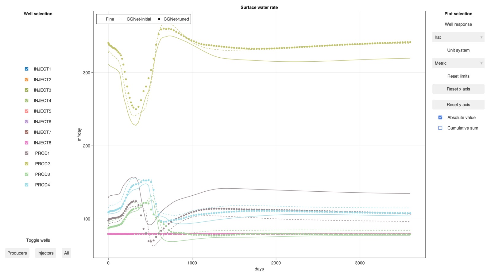

Create a function to compare individual wells

We next compare individual wells to see how the optimization has affected the match between the coarse scale and fine scale. As we can see, we have reasonably good match between the original model with about 18,000 cells and the coarse model with about 3000 cells. Even better match could be possible by adding more coarse blocks, or also optimizing for example the relative permeability parameters for the coarse model.

We plot the water cut and total rate for the production wells, and the bottom hole pressure for the injection wells.

julia

function plot_tuned_well(k, kw; lposition = :lt)
    fig = Figure()
    ax = Axis(fig[1, 1], title = "$k", xlabel = "days", ylabel = "$kw")
    t = wells_f.time./si_unit(:day)
    if kw == :wcut
        F = x -> x[k, :wrat]./x[k, :lrat]
    else
        F = x -> abs.(x[k, kw])
    end

    lines!(ax, t, F(wells_f), label = "Fine-scale")
    lines!(ax, t, F(wells_c), label = "Initial coarse")
    lines!(ax, t, F(wells_t), label = "Tuned coarse")
    axislegend(position = lposition)
    fig
end

plot_tuned_well (generic function with 1 method)

Plot PROD1 water cut

julia

plot_tuned_well(:PROD1, :wcut)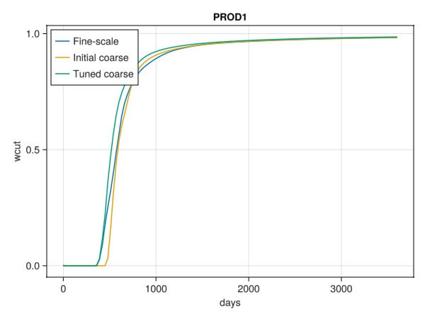

Plot PROD2 water cut

julia

plot_tuned_well(:PROD2, :wcut)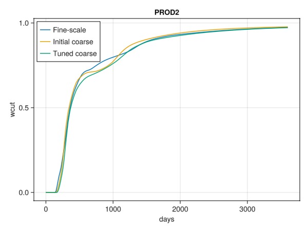

Plot PROD4 water cut

julia

plot_tuned_well(:PROD4, :wcut)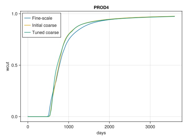

Plot PROD1 total rate

julia

plot_tuned_well(:PROD1, :rate)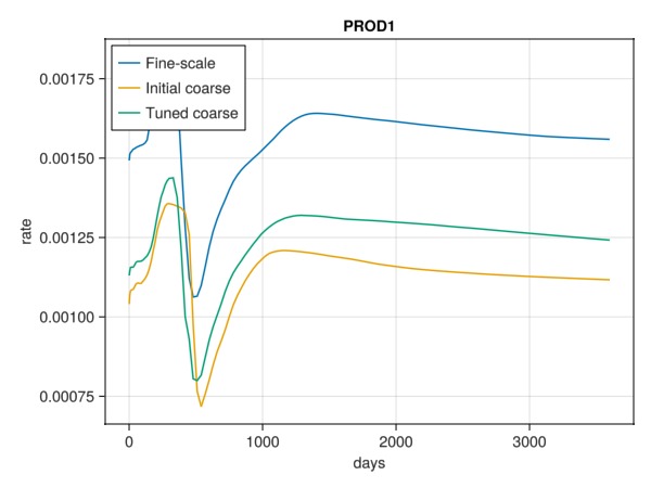

Plot PROD2 total rate

julia

plot_tuned_well(:PROD2, :rate)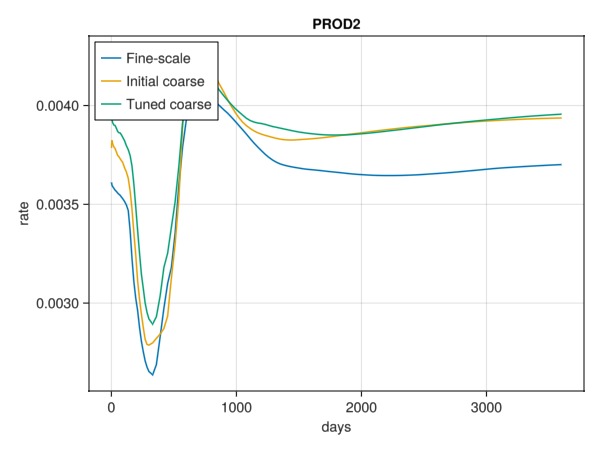

Plot PROD4 total rate

julia

plot_tuned_well(:PROD4, :rate)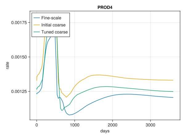

Plot INJECT1 bhp

julia

plot_tuned_well(:INJECT1, :bhp, lposition = :rt)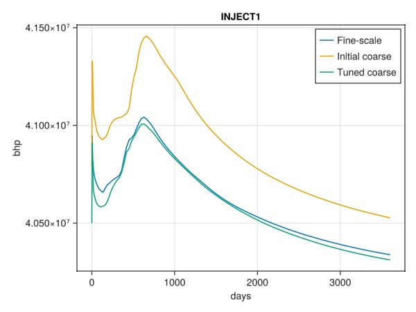

Plot INJECT4 bhp

julia

plot_tuned_well(:INJECT4, :bhp, lposition = :rt)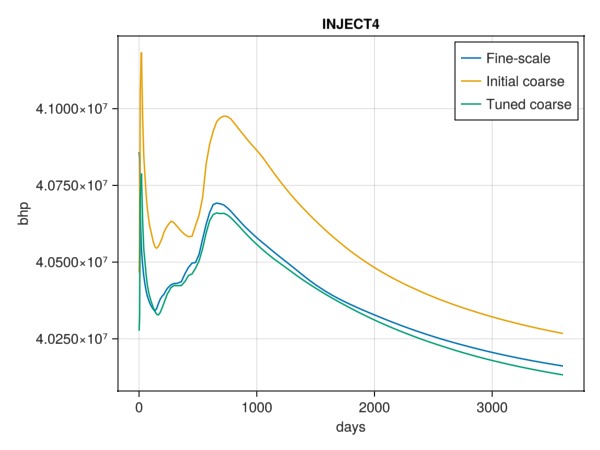

Plot the objective evaluations during optimization

julia

fig = Figure()
ys = log10
is = x -> x
ax1 = Axis(fig[1, 1], yscale = ys, title = "Objective evaluations", xlabel = "Iterations", ylabel = "Objective")
plot!(ax1, opt_setup[:data][:obj_hist][2:end])
fig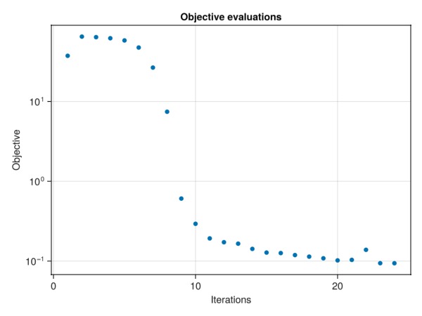

Plot the evoluation of scaled parameters

We show the difference between the initial and final values of the scaled parameters, as well as the lower bound.

JutulDarcy maps the parameters to a single vector for optimization with values that are approximately in the box limit range (0, 1). This is convenient for optimizers, but can also be useful when plotting the parameters, even if the units are not preserved in this visualization, only the magnitude.

julia

fig = Figure(size = (800, 600))
ax1 = Axis(fig[1, 1], title = "Scaled parameters", ylabel = "Scaled value")
scatter!(ax1, setup[:x0], label = "Initial X")
scatter!(ax1, final_x, label = "Final X", markersize = 5)
lines!(ax1, setup[:lower], label = "Lower bound")
axislegend()

trans = data[:mapper][:Reservoir][:Transmissibilities]

function plot_bracket(v, k)
    start = v.offset+1
    stop = v.offset+v.n
    y0 = setup[:lower][start]
    y1 = setup[:lower][stop]
    bracket!(ax1, start, y0, stop, y1,
    text = "$k", offset = 1, orientation = :down)
end

for (k, v) in pairs(data[:mapper][:Reservoir])
    plot_bracket(v, k)
end
ylims!(ax1, (-0.2*maximum(final_x), nothing))
fig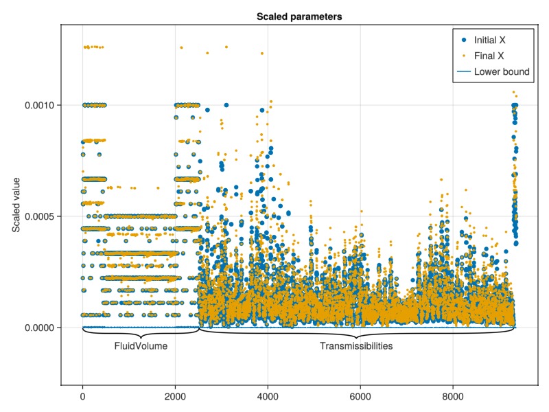

Example on GitHub

If you would like to run this example yourself, it can be downloaded from the JutulDarcy.jl GitHub repository as a script, or as a Jupyter Notebook

This page was generated using Literate.jl.

History matching a coarse model - CGNet ​

Load and simulate Egg base case ​

Create initial coarse model and simulate ​

Setup optimization ​

Define the optimization loop ​

Run the optimization ​

Transfer the results back ​

Plot the results interactively ​

Create a function to compare individual wells ​

Plot PROD1 water cut ​

Plot PROD2 water cut ​

Plot PROD4 water cut ​

Plot PROD1 total rate ​

Plot PROD2 total rate ​

Plot PROD4 total rate ​

Plot INJECT1 bhp ​

Plot INJECT4 bhp ​

Plot the objective evaluations during optimization ​

Plot the evoluation of scaled parameters ​

Example on GitHub ​

History matching a coarse model - CGNet

Load and simulate Egg base case

Create initial coarse model and simulate

Setup optimization

Define the optimization loop

Run the optimization

Transfer the results back

Plot the results interactively

Create a function to compare individual wells

Plot PROD1 water cut

Plot PROD2 water cut

Plot PROD4 water cut

Plot PROD1 total rate

Plot PROD2 total rate

Plot PROD4 total rate

Plot INJECT1 bhp

Plot INJECT4 bhp

Plot the objective evaluations during optimization

Plot the evoluation of scaled parameters

Example on GitHub