Gravity circulation with CPR preconditioner
This example demonstrates a more complex gravity driven instability. The problem is a bit larger than the Gravity segregation example, and is therefore set up using the high level API that automatically sets up an iterative linear solver with a constrained pressure residual (CPR) preconditioner and automatic timestepping.
The high level API uses the more low level Jutul API seen in the other examples under the hood and makes more complex problems easy to set up. The same data structures and functions are used, allowing for deep customization if the defaults are not appropriate.
using JutulDarcy
using Jutul
using CairoMakie
cmap = :seismic
nx = nz = 100;
Define the domain
D = 10.0
g = CartesianMesh((nx, 1, nz), (D, 1.0, D))
domain = reservoir_domain(g)
DataDomain wrapping CartesianMesh (3D) with 100x1x100=10000 cells with 17 data fields added:
10000 Cells
:permeability => 10000 Vector{Float64}
:porosity => 10000 Vector{Float64}
:rock_thermal_conductivity => 10000 Vector{Float64}
:fluid_thermal_conductivity => 10000 Vector{Float64}
:rock_density => 10000 Vector{Float64}
:cell_centroids => 3×10000 Matrix{Float64}
:volumes => 10000 Vector{Float64}
19800 Faces
:neighbors => 2×19800 Matrix{Int64}
:areas => 19800 Vector{Float64}
:normals => 3×19800 Matrix{Float64}
:face_centroids => 3×19800 Matrix{Float64}
39600 HalfFaces
:half_face_cells => 39600 Vector{Int64}
:half_face_faces => 39600 Vector{Int64}
20400 BoundaryFaces
:boundary_areas => 20400 Vector{Float64}
:boundary_centroids => 3×20400 Matrix{Float64}
:boundary_normals => 3×20400 Matrix{Float64}
:boundary_neighbors => 20400 Vector{Int64}
Set up model and properties
Darcy, bar, kg, meter, day = si_units(:darcy, :bar, :kilogram, :meter, :day)
p0 = 100*bar
rhoLS = 1000.0*kg/meter^3 # Definition of fluid phases
rhoVS = 500.0*kg/meter^3
cl, cv = 1e-5/bar, 1e-4/bar
L, V = LiquidPhase(), VaporPhase()
sys = ImmiscibleSystem([L, V])
model, parameters = setup_reservoir_model(domain, sys)
density = ConstantCompressibilityDensities(sys, p0, [rhoLS, rhoVS], [cl, cv]) # Replace density with a lighter pair
replace_variables!(model, PhaseMassDensities = density);
kr = BrooksCoreyRelativePermeabilities(sys, [2.0, 3.0])
replace_variables!(model, RelativePermeabilities = kr)
MultiModel with 1 models and 0 cross-terms. 20000 equations and 20000 degrees of freedom.
models:
1) Reservoir (20000x20000)
ImmiscibleSystem with LiquidPhase, VaporPhase
∈ MinimalTPFATopology (10000 cells, 19800 faces)
Model storage will be optimized for compilation performance.
Define initial saturation
Set the left part of the domain to be filled by the vapor phase and the heavy liquid phase in the remainder. To do this, we grab the cell centroids in the x direction from the domain, reshape them to the structured mesh we are working on and define the liquid saturation from there.
c = domain[:cell_centroids]
x = reshape(c[1, :], nx, nz)

sL = zeros(nx, nz)
plane = D/2.0
for i in 1:nx
    for j = 1:nz
        X = x[i, j]
        sL[i, j] = clamp(Float64(X > plane), 0, 1)
    end
end
heatmap(sL, colormap = cmap, axis = (title = "Initial saturation",))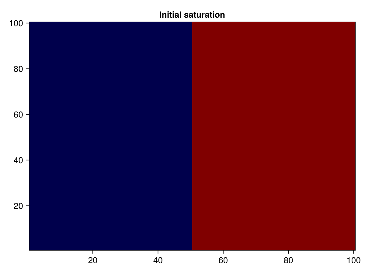
Set up initial state
sL = vec(sL)'
sV = 1 .- sL
s0 = vcat(sV, sL)
state0 = setup_reservoir_state(model, Pressure = p0, Saturations = s0)
Dict{Any, Any} with 1 entry:
:Reservoir => Dict{Symbol, Any}(:PhaseMassMobilities=>[0.0 0.0 … 0.0 0.0; 0.0…Set the viscosity of the phases
By default, viscosity is a parameter and can be set per-phase and per cell.
μ = parameters[:Reservoir][:PhaseViscosities]
@. μ[1, :] = 1e-3
@. μ[2, :] = 5e-3
10000-element view(::Matrix{Float64}, 2, :) with eltype Float64:
0.005
0.005
0.005
0.005
0.005
0.005
0.005
0.005
0.005
0.005
⋮
0.005
0.005
0.005
0.005
0.005
0.005
0.005
0.005
0.005Convert time-steps from days to seconds
timesteps = repeat([10.0*3600*24], 20)
_, states, = simulate_reservoir(state0, model, timesteps, parameters = parameters, info_level = 1);
Jutul: Simulating 28 weeks, 4 days as 20 report steps
Step 1/20: Solving start to 1 week, 3 days, Δt = 1 week, 3 days
Step 2/20: Solving 1 week, 3 days to 2 weeks, 6 days, Δt = 1 week, 3 days
Step 3/20: Solving 2 weeks, 6 days to 4 weeks, 2 days, Δt = 1 week, 3 days
Step 4/20: Solving 4 weeks, 2 days to 5 weeks, 5 days, Δt = 1 week, 3 days
Step 5/20: Solving 5 weeks, 5 days to 7 weeks, 1 day, Δt = 1 week, 3 days
Step 6/20: Solving 7 weeks, 1 day to 8 weeks, 4 days, Δt = 1 week, 3 days
Step 7/20: Solving 8 weeks, 4 days to 10 weeks, Δt = 1 week, 3 days
Step 8/20: Solving 10 weeks to 11 weeks, 3 days, Δt = 1 week, 3 days
Step 9/20: Solving 11 weeks, 3 days to 12 weeks, 6 days, Δt = 1 week, 3 days
Step 10/20: Solving 12 weeks, 6 days to 14 weeks, 2 days, Δt = 1 week, 3 days
Step 11/20: Solving 14 weeks, 2 days to 15 weeks, 5 days, Δt = 1 week, 3 days
Step 12/20: Solving 15 weeks, 5 days to 17 weeks, 1 day, Δt = 1 week, 3 days
Step 13/20: Solving 17 weeks, 1 day to 18 weeks, 4 days, Δt = 1 week, 3 days
Step 14/20: Solving 18 weeks, 4 days to 20 weeks, Δt = 1 week, 3 days
Step 15/20: Solving 20 weeks to 21 weeks, 3 days, Δt = 1 week, 3 days
Step 16/20: Solving 21 weeks, 3 days to 22 weeks, 6 days, Δt = 1 week, 3 days
Step 17/20: Solving 22 weeks, 6 days to 24 weeks, 2 days, Δt = 1 week, 3 days
Step 18/20: Solving 24 weeks, 2 days to 25 weeks, 5 days, Δt = 1 week, 3 days
Step 19/20: Solving 25 weeks, 5 days to 27 weeks, 1 day, Δt = 1 week, 3 days
Step 20/20: Solving 27 weeks, 1 day to 28 weeks, 4 days, Δt = 1 week, 3 days
Simulation complete: Completed 20 report steps in 7 seconds, 292 milliseconds, 547.1 microseconds and 399 iterations.
╭────────────────┬──────────┬──────────────┬──────────┬──────────╮
│ Iteration type │ Avg/step │ Avg/ministep │ Time per │ Total │
│ │ 20 steps │ 67 ministeps │ ms │ (wasted) │
├────────────────┼──────────┼──────────────┼──────────┼──────────┤
│ Newton │ 19.95 │ 5.95522 │ 18.2771 │ 399 (0) │
│ Linearization │ 23.3 │ 6.95522 │ 15.6492 │ 466 (0) │
│ Linear solver │ 63.7 │ 19.0149 │ 5.7241 │ 1274 (0) │
╰────────────────┴──────────┴──────────────┴──────────┴──────────╯
╭────────────────┬─────────┬────────────┬────────╮
│ Timing type │ Each │ Relative │ Total │
│ │ ms │ Percentage │ s │
├────────────────┼─────────┼────────────┼────────┤
│ Properties │ 0.6644 │ 3.64 % │ 0.2651 │
│ Equations │ 0.6687 │ 4.27 % │ 0.3116 │
│ Assembly │ 1.3214 │ 8.44 % │ 0.6158 │
│ Linear solve │ 9.2759 │ 50.75 % │ 3.7011 │
│ Preconditioner │ 5.5665 │ 30.46 % │ 2.2210 │
│ Update │ 0.1793 │ 0.98 % │ 0.0716 │
│ Convergence │ 0.0966 │ 0.62 % │ 0.0450 │
│ Input/Output │ 0.0154 │ 0.01 % │ 0.0010 │
│ Other │ 0.1512 │ 0.83 % │ 0.0603 │
├────────────────┼─────────┼────────────┼────────┤
│ Total │ 18.2771 │ 100.00 % │ 7.2925 │
╰────────────────┴─────────┴────────────┴────────╯Plot results
Plot initial saturation
tmp = reshape(state0[:Reservoir][:Saturations][1, :], nx, nz)
f = Figure()
ax = Axis(f[1, 1], title = "Before")
heatmap!(ax, tmp, colormap = cmap)
MakieCore.Heatmap{Tuple{Vector{Float32}, Vector{Float32}, Matrix{Float32}}}Plot intermediate saturation
tmp = reshape(states[length(states) ÷ 2][:Saturations][1, :], nx, nz)
ax = Axis(f[1, 2], title = "Half way")
hm = heatmap!(ax, tmp, colormap = cmap)
MakieCore.Heatmap{Tuple{Vector{Float32}, Vector{Float32}, Matrix{Float32}}}Plot final saturation
tmp = reshape(states[end][:Saturations][1, :], nx, nz)
ax = Axis(f[1, 3], title = "After")
hm = heatmap!(ax, tmp, colormap = cmap)
Colorbar(f[1, 4], hm)
f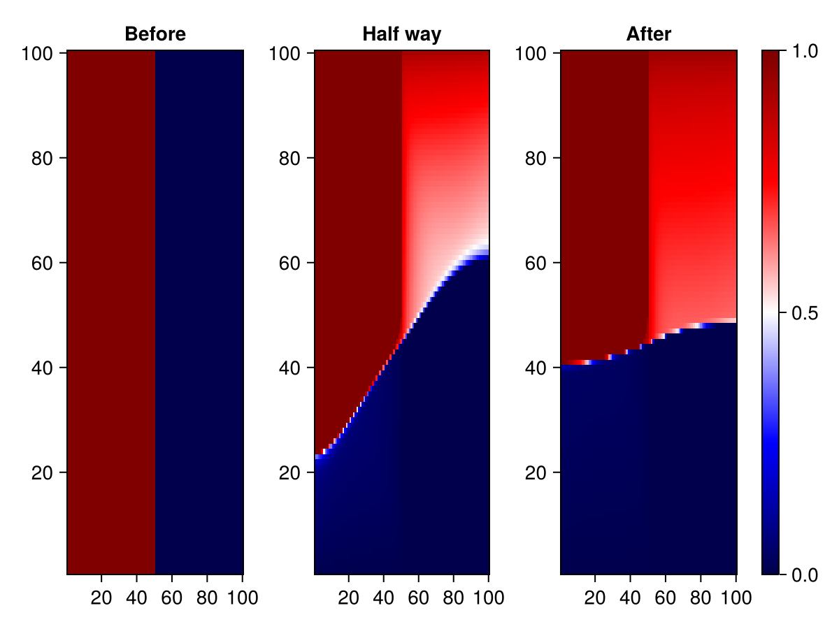
Example on GitHub
If you would like to run this example yourself, it can be downloaded from the JutulDarcy.jl GitHub repository.
This page was generated using Literate.jl.